12 Decision Trees for Machine Learning

Click here to download this chapter as a Jupyter (.ipynb) file.

In this chapter we learn how decision trees may be used for machine learning. A decision tree model may be used for both classification and regression tasks. Models based on decision trees have a few strong advantages. They are fairly easy to visualize and understand, at least for smaller trees, and there is no need to scale numeric data before fitting a tree-based model. They work well with data that has a mix of categorical and numeric features.

12.0.1 Module and Function Imports

import mglearn 
import numpy as np
import pandas as pd
from matplotlib import pyplot as plt
import time

from sklearn.model_selection import train_test_split, RepeatedStratifiedKFold
from sklearn.model_selection import GridSearchCV, cross_validate

from sklearn.datasets import load_breast_cancer
from sklearn.datasets import make_moons

from sklearn.tree import DecisionTreeClassifier

from sklearn.compose import ColumnTransformer
from sklearn.pipeline import Pipeline
from sklearn.preprocessing import OneHotEncoder

from sklearn.tree import export_graphviz

12.1 Decision Trees

A decision tree is a hierarchy of if/else questions, leading to a decision. For example, consider a classification task in which we are trying to classify animals as various species depending on their characteristics, such as if they have feathers, if they can fly, and if they have fins. the decision tree shown below could be used to do the classification. We start at the top of the tree and ask questions as we go down. After each question the data is split into two directions, based on the answer to the question. Each instance in the data will end up at one leaf at the bottom row of the tree, and we can classify the species of that instance based on where it ends up at the bottom of the tree.

mglearn.plots.plot_animal_tree()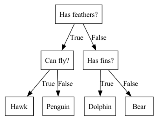

12.1.1 Some tree vocabulary

Before we continue with our exploration of tree-based models we should learn some basic vocabulary related to these models. Each point in the tree at which a splitting decision could be made is called a node. Nodes at the bottom of the tree are called leaf nodes or leaves. The tree can be described by its depth. The depth is the number of splits it takes to reach the lowest leaf node(s) from the top level

12.1.2 How does the tree determine how to split at each node?

Note that there are many specific implementations of decision trees, all of which use slightly different algorithms. The explanation provided below is a generic explanation that applies to most decision tree implementations.

The goal of a decision tree is to recursively split the dataset into subsets that are as homogeneous as possible with respect to the target variable. For example, if we start with 50 instances of data in which 25 instances have the target variable value ‘malignant’ and 25 instances have the target variable value ‘benign’, a split that resulted in all the ‘malignant’ instances on one side of the split and all the ‘benign’ instances on the other side of the split would be a perfect split, because the two leaves that resulted from the split are both homogeneous with respect to the target variable. It would be very unusual to encounter such a perfect split in a real classification task, but we can use that extreme example to understand the general concept; the more homogeneous the leaves resulting from the split are the better the split is considered to be. Another term for homogeneity is purity. At each node the tree-building algorithm finds the split that results in the greatest weighted average purity of the resulting leaves. There are several different ways that purity or impurity can be measured. Two common measures of impurity are Gini impurity and entropy. You may also encounter the term information gain which refers to a reduction in entropy.

Let’s take a closer look at Gini impurity. For binary classification, Gini impurity ranges from 0 to 0.5, where 0 represents pure nodes (all instances in the node belong to the same class), and 0.5 represents maximum impurity (an equal distribution of instances across all classes). It is calculated for a node as as 1 minus the sum of squared class proportions with the following formula, where \(k\) is the number of classes and \(p_i\) is the proportion of class \(i\) in the node: \[G = 1 - \sum_{i=1}^{k} {p_i}^2\]

To find the best split at each node the tree algorithm considers all the possible splits for each feature and selects the split that reduces impurity the most. This process continues recursively until a stopping criterion is met, such as reaching a maximum tree depth, having a minimum number of instances in a leaf node, or when further splits do not reduce impurity by more than a minimum threshold.

The decision tree-building process is essentially a greedy algorithm, making locally optimal choices at each node. Note that this might not always result in the optimal tree structure at a global level.

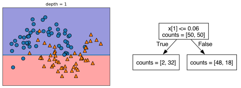
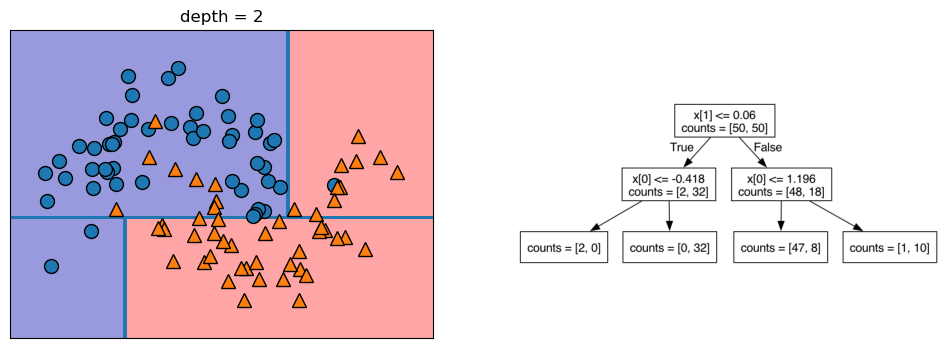
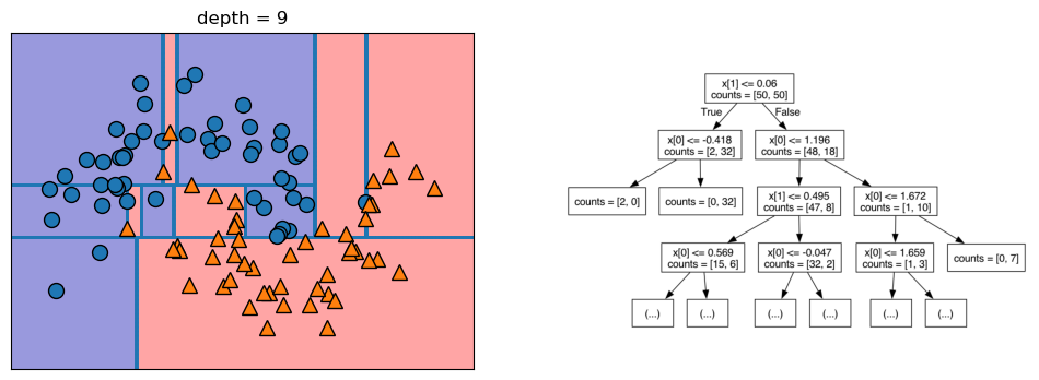
12.1.3 Visualization of a Tree-Based Binary Classification Model with 2 Features

Let’s take a look at some visualizations that show what happens in the first several splits of a tree-building process. We begin by visualizing the data. There are two features, and the target variable has two classes, blue circles and orange triangles. The next few visualizations show the decision boundary created by each split and the current state of the decision tree after each split. Note how adding levels to the tree allows the tree more flexibility to fit the training data. Consider how that will affect generalization performance.

mglearn.plots.plot_tree_progressive()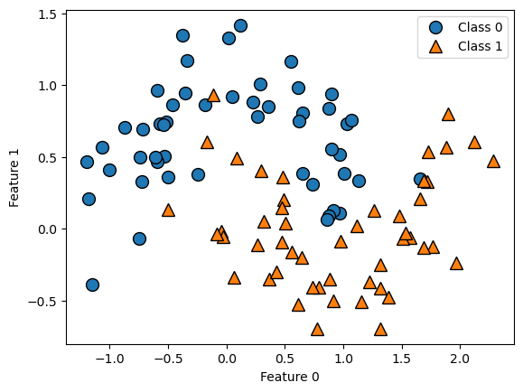

12.1.4 Controlling the Complexity of Decision Trees

If a decision tree model is permitted to continue to split leaves it attempt to keep splitting until all the leaves are pure. So, the more freedom we give the tree to continue to split leaves and grow, the more flexibility we are giving it to fit the training data. We can control the flexibility of decision trees with pre-pruning or post-pruning. Pre-pruning refers to setting some parameter that causes the tree to stop growing at some pre-defined threshold. Following are some commonly-used pre-pruning parameters (see the scikit-learn documentation for others): * max_depth - maximum number of levels for the tree * max_leaf_nodes - maximum number of leaf nodes * min_samples_leaf - stops the splitting when either of the leaves resulting from the split would have fewer than this number of instances in it * min_samples_split - will not split a leaf with fewer than this number of instances in it

When we build single-tree models with scikit-learn we will vary one or more of these parameters to modify the model’s flexibility to fit the training data.

There are also approaches that utilize post-pruning. With post-pruning approaches the full tree is built and then some nodes are removed or collapsed according to some criterion. We will not be covering post-pruning approaches in this chapter.

The primary purpose of both pre-pruning and post-pruning is to limit the complexity (flexibility) of the tree so that it does not overfit the training data.

12.1.5 Estimate Generalization Performance for and Tune the Decision Tree model

Let’s run through the full model-building process for the decision tree algorithm on the Titanic data, tuning the min_samples_leaf parameter:

set up a grid search
run the grid search once to see if parameter range selected is reasonable
run a nested cross validation to estimate generalization performance. Recall that a nested cross validation is a cross validation that uses a grid search as the estimator. It is considered the best way to estimate a model’s generalization performance. Note that it cannot be used to tune the parameters of the final model, however, because each of the interior grid searches may arrive at different settings for the parameters. Because of this, a nested cross validation is typically used to select the best algorithm for the model (tree, logistic regression, K-nn, etc.) and then a separate grid search is performed on the best algorithm using all the data to set the final model parameters
perform final grid search on all the data to tune the model

12.1.6 Load the Titanic Data

In the cell below we will import a subset of the Titanic data, which describes passengers on the Titanic. Below is a brief description of the variables: * Survived - the target variable. Has values 0 or 1, with 1 representing that the passenger survived the disaster * Pclass - represents class of ticket * Sex - represents the sex of the passenger * Age - represents the age of the passenger * SibSp - represents number of siblings or spouse traveling with the passenger * Parch - represents the number of parents or children traveling with the passenger * Embarked - represents the port from which the passenger embarked.

Note: This is only a subset of the actual Titanic dataset.

titanic = pd.read_csv('https://neuronjolt.com/data/titanic.csv')

titanic.info()

<class 'pandas.core.frame.DataFrame'>
RangeIndex: 712 entries, 0 to 711
Data columns (total 7 columns):
 #   Column    Non-Null Count  Dtype  
---  ------    --------------  -----  
 0   Survived  712 non-null    int64  
 1   Pclass    712 non-null    int64  
 2   Sex       712 non-null    object 
 3   Age       712 non-null    float64
 4   SibSp     712 non-null    int64  
 5   Parch     712 non-null    int64  
 6   Embarked  712 non-null    object 
dtypes: float64(1), int64(4), object(2)
memory usage: 39.1+ KB

X = titanic.drop(columns = 'Survived')
y = titanic['Survived']

12.1.7 Define the grid search

The Titanic dataset has both numeric and categorical features. We don’t need to scale the numeric features, as we do with K-nn or linear models, but we do need to one-hot encode the categorical features. So, we will build a column transformer to one-hot encode the categorical features. Note that if we don’t specify an operation to perform on the numeric columns they will be dropped from the analysis unless we explicitly tell the column transformer to pass them through unchanged. We can do that by setting the remainder parameter to 'passthrough' within the ColumnTransformer() function.

Since there are not many rows of data, we will use 3 x stratified 10-fold cross validation as our splitting strategy. We set the n_jobs parameter to -1, which tells scikit learn to parallelize the grid search over all available processor cores.

# Define column transformer to one-hot encode the categorical features
# and pass through the numeric features
ct_dt = ColumnTransformer([
    ('ohe', OneHotEncoder(handle_unknown = 'ignore'), ['Sex', 'Pclass', 'Embarked'])
], remainder = 'passthrough')

# Combine the column transformer with the estimator in a pipeline
pipe_dt = Pipeline([
    ('pre', ct_dt),
    ('dt', DecisionTreeClassifier())
])

# Define the parameter grid
pgrid_dt = {'dt__min_samples_leaf': range(1, 102, 5)}

# Define a custom splitter to do 3 x stratified 10-fold cv
rskf_3x10 = RepeatedStratifiedKFold(n_splits = 10, n_repeats = 3)

# Define the grid search
gs_dt = GridSearchCV(estimator = pipe_dt,
                     param_grid = pgrid_dt,
                     cv = rskf_3x10,
                     n_jobs = -1,
                     return_train_score = True)

12.1.8 Run the grid search once to check parameter range

In the initial grid search we are varying the parameter min_samples_leaf from 1 to 101 by 5s. This parameter controls how far the tree can keep splitting, because a split will not be done if it would result in a leaf with fewer instances in it than the min_samples_leaf setting. The choice of 1 to 101 was made to get a fairly wide range, but go by 5s so the initial grid search doesn’t take too long. We will run the grid search once to see if this parameter range is appropriate. For the grid search we use in the nested cross validation below we want to use a parameter range centered around the best parameter setting from this initial grid search, but if the best parameter setting from the initial grid search is at the high end of the range we should extend the range and try again.

gs_dt.fit(X, y)

GridSearchCV(cv=RepeatedStratifiedKFold(n_repeats=3, n_splits=10, random_state=None),
             estimator=Pipeline(steps=[('pre',
                                        ColumnTransformer(remainder='passthrough',
                                                          transformers=[('ohe',
                                                                         OneHotEncoder(handle_unknown='ignore'),
                                                                         ['Sex',
                                                                          'Pclass',
                                                                          'Embarked'])])),
                                       ('dt', DecisionTreeClassifier())]),
             n_jobs=-1, param_grid={'dt__min_samples_leaf': range(1, 102, 5)},
             return_train_score=True)

In a Jupyter environment, please rerun this cell to show the HTML representation or trust the notebook.
On GitHub, the HTML representation is unable to render, please try loading this page with nbviewer.org.

gs_dt.best_params_

{'dt__min_samples_leaf': 6}

We used the best_params_ property of the fitted grid search object to see what the grid search identified as the best parameter setting for min_samples_leaf. It found that 6 was the best parameter setting. This suggests that our range of 1 to 101 might be a bit wide, because the best parameter setting found on the initial grid search was near the low end of that range. However, before we proceed to the nested cross validation to estimate generalization performance for the decision tree model on the breast cancer data we will create a validation curve plot to see the pattern of how test performance varies with changes in the min_samples_leaf parameter.

# Put the results from the grid search into a DataFrame
results = pd.DataFrame(gs_dt.cv_results_)

# Make the validation curve plot
plt.plot(results['param_dt__min_samples_leaf'], 
         results['mean_train_score'], 
         label="training accuracy")
plt.plot(results['param_dt__min_samples_leaf'],
         results['mean_test_score'],
         label="test accuracy")
plt.axhline(max(results['mean_test_score']), linestyle='dotted', color='gray')
plt.axvline(results['param_dt__min_samples_leaf'].iloc[results['mean_test_score'].idxmax()], 
            linestyle='dotted', color='gray')
plt.title("Validation Curve Graph for Decision Tree")
plt.ylabel("Prediction Accuracy")
plt.xlabel("Min Samples per Leaf")
plt.xlim(max(results['param_dt__min_samples_leaf']), min(results['param_dt__min_samples_leaf']))
plt.legend();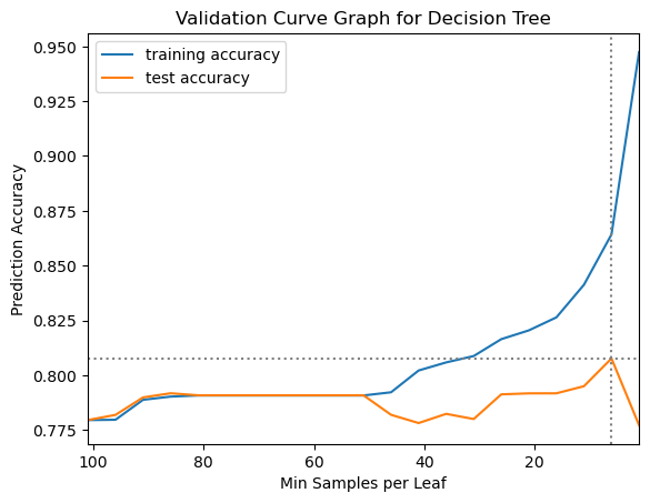

12.1.9 Revise Parameter Grid and Re-Define Grid Search before Nested Cross Validation

We can see from the validation curve plot that the mean test performance from the grid search has its peak at a min_samples_leaf parameter setting of 6 and then declines sharply. To help the nested cross validation run faster we will narrow the range of the parameter grid before running the nested cross validation. Having fewer parameter settings for each grid search to check will take less time, but we don’t want to narrow the range too much, though, because we want to make sure we find the best parameter setting at each split. We will also not save training scores for the nested cross validation. This will also help the grid search to run a bit faster. When we change the parameter grid we need to re-define the grid search as well, to pull in the new parameter grid.

# Re-define the parameter grid
pgrid_dt = {'dt__min_samples_leaf': range(1, 16)}

# Re-define the grid search with the narrowed parameter grid
gs_dt = GridSearchCV(estimator = pipe_dt,
                     param_grid = pgrid_dt,
                     cv = rskf_3x10,
                     n_jobs = -1)

12.1.10 Perform the Nested Cross Validation: Use the grid search as the estimator in a cross validation

For the nested cross validation we will use stratified 10-fold cross validation. Note that we do not set the n_jobs parameter within the cross_validate function below, because it is already set in the grid search that serves as the estimator in the cross_validate function. It is recommended to only set the n_jobs parameter in one level of a nested grid search, either in the grid search or the cross validate but not both.

# Perform the nested cross validation
results_dt = cross_validate(estimator = gs_dt,
                            X = X,
                            y = y,
                            cv = 10)

12.1.10.1 Calculate the mean test score as estimate of generalization performance

Below we calculate the mean score on the test folds from the nested cross validation. This is our best estimate of the generalization performance of the decision tree model on the breast cancer data. It is also useful to take a look at the standard deviation of the test score to see how sensitive the test scores are to the data splits.

results_dt['test_score'].mean()

np.float64(0.7894757433489827)

results_dt['test_score'].std()

np.float64(0.05903215268777309)

So, our estimate of the generalization performance of the decision tree model on the Titanic data is around 79% accuracy, with a standard deviation of around 6%.

In a full model building process we would perform nested cross validation for each algorithm we were considering (K-nn, logistic regression, decision tree, etc.) to determine which algorithm has the best estimated generalization performance on our data. Then, we would re-run the grid search for the best algorithm on the unsplit data to tune it and prepare it to make future predictions.

final_model = gs_dt.fit(X, y)

If we had new data, we would use this final model’s predict method to make predictions of the target variable, with code such as the following:
preds = final_model.predict(new_data)

	estimator estimator: estimator object This is assumed to implement the scikit-learn estimator interface. Either estimator needs to provide a ``score`` function, or ``scoring`` must be passed.	Pipeline(step...lassifier())])
	param_grid param_grid: dict or list of dictionaries Dictionary with parameters names (`str`) as keys and lists of parameter settings to try as values, or a list of such dictionaries, in which case the grids spanned by each dictionary in the list are explored. This enables searching over any sequence of parameter settings.	{'dt__min_samples_leaf': range(1, 102, 5)}
	scoring scoring: str, callable, list, tuple or dict, default=None Strategy to evaluate the performance of the cross-validated model on the test set. If `scoring` represents a single score, one can use: - a single string (see :ref:`scoring_string_names`); - a callable (see :ref:`scoring_callable`) that returns a single value; - `None`, the `estimator`'s :ref:`default evaluation criterion ` is used. If `scoring` represents multiple scores, one can use: - a list or tuple of unique strings; - a callable returning a dictionary where the keys are the metric names and the values are the metric scores; - a dictionary with metric names as keys and callables as values. See :ref:`multimetric_grid_search` for an example.	None
	n_jobs n_jobs: int, default=None Number of jobs to run in parallel. ``None`` means 1 unless in a :obj:`joblib.parallel_backend` context. ``-1`` means using all processors. See :term:`Glossary ` for more details. .. versionchanged:: v0.20 `n_jobs` default changed from 1 to None	-1
	refit refit: bool, str, or callable, default=True Refit an estimator using the best found parameters on the whole dataset. For multiple metric evaluation, this needs to be a `str` denoting the scorer that would be used to find the best parameters for refitting the estimator at the end. Where there are considerations other than maximum score in choosing a best estimator, ``refit`` can be set to a function which returns the selected ``best_index_`` given ``cv_results_``. In that case, the ``best_estimator_`` and ``best_params_`` will be set according to the returned ``best_index_`` while the ``best_score_`` attribute will not be available. The refitted estimator is made available at the ``best_estimator_`` attribute and permits using ``predict`` directly on this ``GridSearchCV`` instance. Also for multiple metric evaluation, the attributes ``best_index_``, ``best_score_`` and ``best_params_`` will only be available if ``refit`` is set and all of them will be determined w.r.t this specific scorer. See ``scoring`` parameter to know more about multiple metric evaluation. See :ref:`sphx_glr_auto_examples_model_selection_plot_grid_search_digits.py` to see how to design a custom selection strategy using a callable via `refit`. See :ref:`this example ` for an example of how to use ``refit=callable`` to balance model complexity and cross-validated score. .. versionchanged:: 0.20 Support for callable added.	True
	cv cv: int, cross-validation generator or an iterable, default=None Determines the cross-validation splitting strategy. Possible inputs for cv are: - None, to use the default 5-fold cross validation, - integer, to specify the number of folds in a `(Stratified)KFold`, - :term:`CV splitter`, - An iterable yielding (train, test) splits as arrays of indices. For integer/None inputs, if the estimator is a classifier and ``y`` is either binary or multiclass, :class:`StratifiedKFold` is used. In all other cases, :class:`KFold` is used. These splitters are instantiated with `shuffle=False` so the splits will be the same across calls. Refer :ref:`User Guide ` for the various cross-validation strategies that can be used here. .. versionchanged:: 0.22 ``cv`` default value if None changed from 3-fold to 5-fold.	RepeatedStrat...om_state=None)
	verbose verbose: int Controls the verbosity: the higher, the more messages. - >1 : the computation time for each fold and parameter candidate is displayed; - >2 : the score is also displayed; - >3 : the fold and candidate parameter indexes are also displayed together with the starting time of the computation.	0
	pre_dispatch pre_dispatch: int, or str, default='2n_jobs' Controls the number of jobs that get dispatched during parallel execution. Reducing this number can be useful to avoid an explosion of memory consumption when more jobs get dispatched than CPUs can process. This parameter can be: - None, in which case all the jobs are immediately created and spawned. Use this for lightweight and fast-running jobs, to avoid delays due to on-demand spawning of the jobs - An int, giving the exact number of total jobs that are spawned - A str, giving an expression as a function of n_jobs, as in '2n_jobs'	'2*n_jobs'
	error_score error_score: 'raise' or numeric, default=np.nan Value to assign to the score if an error occurs in estimator fitting. If set to 'raise', the error is raised. If a numeric value is given, FitFailedWarning is raised. This parameter does not affect the refit step, which will always raise the error.	nan
	return_train_score return_train_score: bool, default=False If ``False``, the ``cv_results_`` attribute will not include training scores. Computing training scores is used to get insights on how different parameter settings impact the overfitting/underfitting trade-off. However computing the scores on the training set can be computationally expensive and is not strictly required to select the parameters that yield the best generalization performance. .. versionadded:: 0.19 .. versionchanged:: 0.21 Default value was changed from ``True`` to ``False``	True

	transformers transformers: list of tuples List of (name, transformer, columns) tuples specifying the transformer objects to be applied to subsets of the data. name : str Like in Pipeline and FeatureUnion, this allows the transformer and its parameters to be set using ``set_params`` and searched in grid search. transformer : {'drop', 'passthrough'} or estimator Estimator must support :term:`fit` and :term:`transform`. Special-cased strings 'drop' and 'passthrough' are accepted as well, to indicate to drop the columns or to pass them through untransformed, respectively. columns : str, array-like of str, int, array-like of int, array-like of bool, slice or callable Indexes the data on its second axis. Integers are interpreted as positional columns, while strings can reference DataFrame columns by name. A scalar string or int should be used where ``transformer`` expects X to be a 1d array-like (vector), otherwise a 2d array will be passed to the transformer. A callable is passed the input data `X` and can return any of the above. To select multiple columns by name or dtype, you can use :obj:`make_column_selector`.	[('ohe', ...)]
	remainder remainder: {'drop', 'passthrough'} or estimator, default='drop' By default, only the specified columns in `transformers` are transformed and combined in the output, and the non-specified columns are dropped. (default of ``'drop'``). By specifying ``remainder='passthrough'``, all remaining columns that were not specified in `transformers`, but present in the data passed to `fit` will be automatically passed through. This subset of columns is concatenated with the output of the transformers. For dataframes, extra columns not seen during `fit` will be excluded from the output of `transform`. By setting ``remainder`` to be an estimator, the remaining non-specified columns will use the ``remainder`` estimator. The estimator must support :term:`fit` and :term:`transform`. Note that using this feature requires that the DataFrame columns input at :term:`fit` and :term:`transform` have identical order.	'passthrough'
	sparse_threshold sparse_threshold: float, default=0.3 If the output of the different transformers contains sparse matrices, these will be stacked as a sparse matrix if the overall density is lower than this value. Use ``sparse_threshold=0`` to always return dense. When the transformed output consists of all dense data, the stacked result will be dense, and this keyword will be ignored.	0.3
	n_jobs n_jobs: int, default=None Number of jobs to run in parallel. ``None`` means 1 unless in a :obj:`joblib.parallel_backend` context. ``-1`` means using all processors. See :term:`Glossary ` for more details.	None
	transformer_weights transformer_weights: dict, default=None Multiplicative weights for features per transformer. The output of the transformer is multiplied by these weights. Keys are transformer names, values the weights.	None
	verbose verbose: bool, default=False If True, the time elapsed while fitting each transformer will be printed as it is completed.	False
	verbose_feature_names_out verbose_feature_names_out: bool, str or Callable[[str, str], str], default=True - If True, :meth:`ColumnTransformer.get_feature_names_out` will prefix all feature names with the name of the transformer that generated that feature. It is equivalent to setting `verbose_feature_names_out="{transformer_name}__{feature_name}"`. - If False, :meth:`ColumnTransformer.get_feature_names_out` will not prefix any feature names and will error if feature names are not unique. - If ``Callable[[str, str], str]``, :meth:`ColumnTransformer.get_feature_names_out` will rename all the features using the name of the transformer. The first argument of the callable is the transformer name and the second argument is the feature name. The returned string will be the new feature name. - If ``str``, it must be a string ready for formatting. The given string will be formatted using two field names: ``transformer_name`` and ``feature_name``. e.g. ``"{feature_name}__{transformer_name}"``. See :meth:`str.format` method from the standard library for more info. .. versionadded:: 1.0 .. versionchanged:: 1.6 `verbose_feature_names_out` can be a callable or a string to be formatted.	True
	force_int_remainder_cols force_int_remainder_cols: bool, default=False This parameter has no effect. .. note:: If you do not access the list of columns for the remainder columns in the `transformers_` fitted attribute, you do not need to set this parameter. .. versionadded:: 1.5 .. versionchanged:: 1.7 The default value for `force_int_remainder_cols` will change from `True` to `False` in version 1.7. .. deprecated:: 1.7 `force_int_remainder_cols` is deprecated and will be removed in 1.9.	'deprecated'

	categories categories: 'auto' or a list of array-like, default='auto' Categories (unique values) per feature: - 'auto' : Determine categories automatically from the training data. - list : ``categories[i]`` holds the categories expected in the ith column. The passed categories should not mix strings and numeric values within a single feature, and should be sorted in case of numeric values. The used categories can be found in the ``categories_`` attribute. .. versionadded:: 0.20	'auto'
	drop drop: {'first', 'if_binary'} or an array-like of shape (n_features,), default=None Specifies a methodology to use to drop one of the categories per feature. This is useful in situations where perfectly collinear features cause problems, such as when feeding the resulting data into an unregularized linear regression model. However, dropping one category breaks the symmetry of the original representation and can therefore induce a bias in downstream models, for instance for penalized linear classification or regression models. - None : retain all features (the default). - 'first' : drop the first category in each feature. If only one category is present, the feature will be dropped entirely. - 'if_binary' : drop the first category in each feature with two categories. Features with 1 or more than 2 categories are left intact. - array : ``drop[i]`` is the category in feature ``X[:, i]`` that should be dropped. When `max_categories` or `min_frequency` is configured to group infrequent categories, the dropping behavior is handled after the grouping. .. versionadded:: 0.21 The parameter `drop` was added in 0.21. .. versionchanged:: 0.23 The option `drop='if_binary'` was added in 0.23. .. versionchanged:: 1.1 Support for dropping infrequent categories.	None
	sparse_output sparse_output: bool, default=True When ``True``, it returns a :class:`scipy.sparse.csr_matrix`, i.e. a sparse matrix in "Compressed Sparse Row" (CSR) format. .. versionadded:: 1.2 `sparse` was renamed to `sparse_output`	True
	dtype dtype: number type, default=np.float64 Desired dtype of output.	<class 'numpy.float64'>
	handle_unknown handle_unknown: {'error', 'ignore', 'infrequent_if_exist', 'warn'}, default='error' Specifies the way unknown categories are handled during :meth:`transform`. - 'error' : Raise an error if an unknown category is present during transform. - 'ignore' : When an unknown category is encountered during transform, the resulting one-hot encoded columns for this feature will be all zeros. In the inverse transform, an unknown category will be denoted as None. - 'infrequent_if_exist' : When an unknown category is encountered during transform, the resulting one-hot encoded columns for this feature will map to the infrequent category if it exists. The infrequent category will be mapped to the last position in the encoding. During inverse transform, an unknown category will be mapped to the category denoted `'infrequent'` if it exists. If the `'infrequent'` category does not exist, then :meth:`transform` and :meth:`inverse_transform` will handle an unknown category as with `handle_unknown='ignore'`. Infrequent categories exist based on `min_frequency` and `max_categories`. Read more in the :ref:`User Guide `. - 'warn' : When an unknown category is encountered during transform a warning is issued, and the encoding then proceeds as described for `handle_unknown="infrequent_if_exist"`. .. versionchanged:: 1.1 `'infrequent_if_exist'` was added to automatically handle unknown categories and infrequent categories. .. versionadded:: 1.6 The option `"warn"` was added in 1.6.	'ignore'
	min_frequency min_frequency: int or float, default=None Specifies the minimum frequency below which a category will be considered infrequent. - If `int`, categories with a smaller cardinality will be considered infrequent. - If `float`, categories with a smaller cardinality than `min_frequency * n_samples` will be considered infrequent. .. versionadded:: 1.1 Read more in the :ref:`User Guide `.	None
	max_categories max_categories: int, default=None Specifies an upper limit to the number of output features for each input feature when considering infrequent categories. If there are infrequent categories, `max_categories` includes the category representing the infrequent categories along with the frequent categories. If `None`, there is no limit to the number of output features. .. versionadded:: 1.1 Read more in the :ref:`User Guide `.	None
	feature_name_combiner feature_name_combiner: "concat" or callable, default="concat" Callable with signature `def callable(input_feature, category)` that returns a string. This is used to create feature names to be returned by :meth:`get_feature_names_out`. `"concat"` concatenates encoded feature name and category with `feature + "_" + str(category)`.E.g. feature X with values 1, 6, 7 create feature names `X_1, X_6, X_7`. .. versionadded:: 1.3	'concat'

	criterion criterion: {"gini", "entropy", "log_loss"}, default="gini" The function to measure the quality of a split. Supported criteria are "gini" for the Gini impurity and "log_loss" and "entropy" both for the Shannon information gain, see :ref:`tree_mathematical_formulation`.	'gini'
	splitter splitter: {"best", "random"}, default="best" The strategy used to choose the split at each node. Supported strategies are "best" to choose the best split and "random" to choose the best random split.	'best'
	max_depth max_depth: int, default=None The maximum depth of the tree. If None, then nodes are expanded until all leaves are pure or until all leaves contain less than min_samples_split samples.	None
	min_samples_split min_samples_split: int or float, default=2 The minimum number of samples required to split an internal node: - If int, then consider `min_samples_split` as the minimum number. - If float, then `min_samples_split` is a fraction and `ceil(min_samples_split * n_samples)` are the minimum number of samples for each split. .. versionchanged:: 0.18 Added float values for fractions.	2
	min_samples_leaf min_samples_leaf: int or float, default=1 The minimum number of samples required to be at a leaf node. A split point at any depth will only be considered if it leaves at least ``min_samples_leaf`` training samples in each of the left and right branches. This may have the effect of smoothing the model, especially in regression. - If int, then consider `min_samples_leaf` as the minimum number. - If float, then `min_samples_leaf` is a fraction and `ceil(min_samples_leaf * n_samples)` are the minimum number of samples for each node. .. versionchanged:: 0.18 Added float values for fractions.	6
	min_weight_fraction_leaf min_weight_fraction_leaf: float, default=0.0 The minimum weighted fraction of the sum total of weights (of all the input samples) required to be at a leaf node. Samples have equal weight when sample_weight is not provided.	0.0
	max_features max_features: int, float or {"sqrt", "log2"}, default=None The number of features to consider when looking for the best split: - If int, then consider `max_features` features at each split. - If float, then `max_features` is a fraction and `max(1, int(max_features * n_features_in_))` features are considered at each split. - If "sqrt", then `max_features=sqrt(n_features)`. - If "log2", then `max_features=log2(n_features)`. - If None, then `max_features=n_features`. .. note:: The search for a split does not stop until at least one valid partition of the node samples is found, even if it requires to effectively inspect more than ``max_features`` features.	None
	random_state random_state: int, RandomState instance or None, default=None Controls the randomness of the estimator. The features are always randomly permuted at each split, even if ``splitter`` is set to ``"best"``. When ``max_features < n_features``, the algorithm will select ``max_features`` at random at each split before finding the best split among them. But the best found split may vary across different runs, even if ``max_features=n_features``. That is the case, if the improvement of the criterion is identical for several splits and one split has to be selected at random. To obtain a deterministic behaviour during fitting, ``random_state`` has to be fixed to an integer. See :term:`Glossary ` for details.	None
	max_leaf_nodes max_leaf_nodes: int, default=None Grow a tree with ``max_leaf_nodes`` in best-first fashion. Best nodes are defined as relative reduction in impurity. If None then unlimited number of leaf nodes.	None
	min_impurity_decrease min_impurity_decrease: float, default=0.0 A node will be split if this split induces a decrease of the impurity greater than or equal to this value. The weighted impurity decrease equation is the following:: N_t / N * (impurity - N_t_R / N_t * right_impurity - N_t_L / N_t * left_impurity) where ``N`` is the total number of samples, ``N_t`` is the number of samples at the current node, ``N_t_L`` is the number of samples in the left child, and ``N_t_R`` is the number of samples in the right child. ``N``, ``N_t``, ``N_t_R`` and ``N_t_L`` all refer to the weighted sum, if ``sample_weight`` is passed. .. versionadded:: 0.19	0.0
	class_weight class_weight: dict, list of dict or "balanced", default=None Weights associated with classes in the form ``{class_label: weight}``. If None, all classes are supposed to have weight one. For multi-output problems, a list of dicts can be provided in the same order as the columns of y. Note that for multioutput (including multilabel) weights should be defined for each class of every column in its own dict. For example, for four-class multilabel classification weights should be [{0: 1, 1: 1}, {0: 1, 1: 5}, {0: 1, 1: 1}, {0: 1, 1: 1}] instead of [{1:1}, {2:5}, {3:1}, {4:1}]. The "balanced" mode uses the values of y to automatically adjust weights inversely proportional to class frequencies in the input data as ``n_samples / (n_classes * np.bincount(y))`` For multi-output, the weights of each column of y will be multiplied. Note that these weights will be multiplied with sample_weight (passed through the fit method) if sample_weight is specified.	None
	ccp_alpha ccp_alpha: non-negative float, default=0.0 Complexity parameter used for Minimal Cost-Complexity Pruning. The subtree with the largest cost complexity that is smaller than ``ccp_alpha`` will be chosen. By default, no pruning is performed. See :ref:`minimal_cost_complexity_pruning` for details. See :ref:`sphx_glr_auto_examples_tree_plot_cost_complexity_pruning.py` for an example of such pruning. .. versionadded:: 0.22	0.0
	monotonic_cst monotonic_cst: array-like of int of shape (n_features), default=None Indicates the monotonicity constraint to enforce on each feature. - 1: monotonic increase - 0: no constraint - -1: monotonic decrease If monotonic_cst is None, no constraints are applied. Monotonicity constraints are not supported for: - multiclass classifications (i.e. when `n_classes > 2`), - multioutput classifications (i.e. when `n_outputs_ > 1`), - classifications trained on data with missing values. The constraints hold over the probability of the positive class. Read more in the :ref:`User Guide `. .. versionadded:: 1.4	None