import mglearn
import numpy as np
import pandas as pd
import matplotlib as mpl
import matplotlib.pyplot as plt

from sklearn.model_selection import train_test_split
from sklearn.model_selection import RepeatedStratifiedKFold
from sklearn.model_selection import cross_validate
from sklearn.model_selection import GridSearchCV

from sklearn.datasets import load_digits
from sklearn.datasets import make_blobs

from sklearn.linear_model import LogisticRegression
from sklearn.neighbors import KNeighborsClassifier
from sklearn.tree import DecisionTreeClassifier
from sklearn.ensemble import RandomForestClassifier
from sklearn.dummy import DummyClassifier

from sklearn.metrics import get_scorer_names
from sklearn.metrics import confusion_matrix
from sklearn.metrics import classification_report
from sklearn.metrics import f1_score
from sklearn.metrics import roc_curve
from sklearn.metrics import roc_auc_score
from sklearn.metrics import accuracy_score
from sklearn.metrics import ConfusionMatrixDisplay13 Metrics for Binary Classification
Click here to download this chapter as a Jupyter (.ipynb) file.
This chapter introduces metrics other than simple accuracy that are useful for evaluating binary classification models.
13.1 Module and Function Imports
13.2 What’s Wrong with Using Accuracy as the Performance Metric?
A classification model’s accuracy is calculated as the number of correct predictions divided by the total number of predictions. In other words, accuracy is calculated as 100% minus the percentage of predictions that are mistakes or errors. Accuracy is often not the best metric with which to evaluate binary classifier performance. This is because the accuracy metric treats all errors as being equal, but we know that in many real prediction situations related to binary classification different types of errors are not equal; they have different costs. Conversely, different types of correct predictions have different benefits.
13.2.1 Types of errors
In binary classification we often call the class we are trying to predict the positive class and the other class the negative class. For example, if we were building a model to predict presence of cancer in a tissue sample cancerous would be the positive class and not cancerous would be the negative class. There are two types of binary classification errors:
- False positive or type 1 error - predicting the positive class when the instance is actually a member of the negative class. In the cancer example a false positive would refer to classifying a tumor that is actually benign as a cancerous tumor.
- False negative or type 2 error - predicting the negative class when the instance is actually a member of the positive class. In the cancer example a false negative would refer to classifying a tumor that is actually cancerous as benign.
As you can understand from the cancer example, these two types of errors rarely have the same costs, but accuracy as a metric treats both types of errors equally.
13.2.2 Imbalanced datasets
Datasets with very different percentages of the positive and negative classes are referred to as imbalanced datasets. On highly imbalanced datasets we can achieve high accuracy by simply always predicting the most prevalent class. However, such a model doesn’t do what we want, which is usually to distinguish between the two classes. This is another reason why we might want to use a metric other than accuracy to evaluate our classification models.
13.3 Comparison of the Accuracy of Different Classifiers on the Digits Data
In this section we will use simple accuracy to compare the performance of various classification algorithms on data related to the digits 0 - 9. Later, to highlight the differences among various performance metrics we will use alternative metrics to compare the performance of those same classification algorithms on the digits dataset.
13.3.1 Load the digits data
Let’s load the digits dataset, which has data on images of handwritten digits (0 - 9). The target value is the digit depicted in the image. We will make it a binary classification task by predicting if the digit is a 9.
digits = load_digits()
digits.keys()
dict_keys(['data', 'target', 'frame', 'feature_names', 'target_names', 'images', 'DESCR'])print(digits.DESCR).. _digits_dataset:
Optical recognition of handwritten digits dataset
--------------------------------------------------
**Data Set Characteristics:**
:Number of Instances: 1797
:Number of Attributes: 64
:Attribute Information: 8x8 image of integer pixels in the range 0..16.
:Missing Attribute Values: None
:Creator: E. Alpaydin (alpaydin '@' boun.edu.tr)
:Date: July; 1998
This is a copy of the test set of the UCI ML hand-written digits datasets
https://archive.ics.uci.edu/ml/datasets/Optical+Recognition+of+Handwritten+Digits
The data set contains images of hand-written digits: 10 classes where
each class refers to a digit.
Preprocessing programs made available by NIST were used to extract
normalized bitmaps of handwritten digits from a preprinted form. From a
total of 43 people, 30 contributed to the training set and different 13
to the test set. 32x32 bitmaps are divided into nonoverlapping blocks of
4x4 and the number of on pixels are counted in each block. This generates
an input matrix of 8x8 where each element is an integer in the range
0..16. This reduces dimensionality and gives invariance to small
distortions.
For info on NIST preprocessing routines, see M. D. Garris, J. L. Blue, G.
T. Candela, D. L. Dimmick, J. Geist, P. J. Grother, S. A. Janet, and C.
L. Wilson, NIST Form-Based Handprint Recognition System, NISTIR 5469,
1994.
.. dropdown:: References
- C. Kaynak (1995) Methods of Combining Multiple Classifiers and Their
Applications to Handwritten Digit Recognition, MSc Thesis, Institute of
Graduate Studies in Science and Engineering, Bogazici University.
- E. Alpaydin, C. Kaynak (1998) Cascading Classifiers, Kybernetika.
- Ken Tang and Ponnuthurai N. Suganthan and Xi Yao and A. Kai Qin.
Linear dimensionalityreduction using relevance weighted LDA. School of
Electrical and Electronic Engineering Nanyang Technological University.
2005.
- Claudio Gentile. A New Approximate Maximal Margin Classification
Algorithm. NIPS. 2000.
digits.target.shape(1797,)digits.target[:20]array([0, 1, 2, 3, 4, 5, 6, 7, 8, 9, 0, 1, 2, 3, 4, 5, 6, 7, 8, 9])# Define y as the target variable for a model predicting 9s
y = digits.target == 9
yarray([False, False, False, ..., False, True, False], shape=(1797,))13.3.2 Perform a stratified train-test split
For the purposes of this example we set random_state = 0 within the train_test_split() function so that we all get the same split. In a real analysis, you would rarely want to set the random state.
X_train, X_test, y_train, y_test = train_test_split(digits.data,
                                                    y,
                                                    stratify = y,
                                                    random_state = 0)
# Calculate the percentage of the positive class (9s) in the data
np.mean(y_train == True)np.float64(0.10022271714922049)13.3.3 Investigate simple accuracy of various classification algorithms
The DummyClassifier can be used to predict the most frequent class, or to make random predictions with the same percentages of the positive and negative class as are present in the training data. Such predictions provide a base case to which to compare predictions from our machine learning models.
Let’s first look at simple accuracy for some DummyClassifier methods and other classification methods.
# First try the strategy of predicting the most frequent value
dummy_most_frequent = DummyClassifier(strategy='most_frequent').fit(X_train, y_train)
pred_most_frequent = dummy_most_frequent.predict(X_test)
# Verify that the predictions are all the most frequent class (False)
np.mean(pred_most_frequent == False)np.float64(1.0)# Calculate accuracy of the dummy_most_frequent classifier on the test data
dummy_most_frequent.score(X_test, y_test)0.9# Now try the 'stratified' strategy, which generates predictions randomly
# according to the training set’s class distribution.
dummy_stratified = DummyClassifier(strategy='stratified').fit(X_train, y_train)
pred_stratified = dummy_stratified.predict(X_test)# Calculate accuracy of the dummy_stratified classifier on the test data
dummy_stratified.score(X_test, y_test)0.8044444444444444# Now let's look at a classification tree, with max_depth set to 3.
tree = DecisionTreeClassifier(max_depth = 3).fit(X_train, y_train)
pred_tree = tree.predict(X_test)
tree.score(X_test, y_test)0.9511111111111111# Let's try logistic regression with the regularization parameter C set
# to 0.1. The strength of regularization is inversely proportional to `C`, so
# higher values of C results in less regularization.
logreg = LogisticRegression(C = 0.1, max_iter = 3_000).fit(X_train, y_train)
pred_logreg = logreg.predict(X_test)
logreg.score(X_test, y_test)0.982222222222222213.4 Confusion Matrices
Confusion matrices are a tool that help us to evaluate binary classifier performance by splitting out counts of the various types of correct decisions and errors made. Confusion matrices for binary classification are a 2z2 matrix.
13.4.1 Graph of Counts of Correct Predictions and Errors on Confusion Matrix
plt.figure(figsize=(6, 5))
confusion = np.array([[401, 2], [8, 39]])
plt.text(0.40, .7, confusion[0, 0], size=50, horizontalalignment='right')
plt.text(0.40, .2, confusion[1, 0], size=50, horizontalalignment='right')
plt.text(.90, .7, confusion[0, 1], size=50, horizontalalignment='right')
plt.text(.90, 0.2, confusion[1, 1], size=50, horizontalalignment='right')
plt.xticks([.25, .75], ["pred 'not nine'", "pred 'nine'"], size=16)
plt.yticks([.25, .75], ["true 'nine'", "true 'not nine'"], size=16)
plt.plot([.5, .5], [0, 1], '--', c='k')
plt.plot([0, 1], [.5, .5], '--', c='k')

plt.xlim(0, 1)
plt.ylim(0, 1);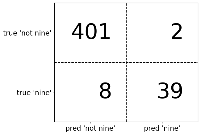
13.4.2 Graph of Types of Errors and Correct Predictions on Confusion Matrix
plt.figure(figsize=(6, 5))

plt.text(0.35, .65, "TN", size=70, horizontalalignment='right')
plt.text(0.35, .15, "FN", size=70, horizontalalignment='right')
plt.text(.85, .65, "FP", size=70, horizontalalignment='right')
plt.text(.85, .15, "TP", size=70, horizontalalignment='right')
plt.xticks([.25, .75], ["predicted negative", "predicted positive"], size=15)
plt.yticks([.25, .75], ["positive class", "negative class"], size=15)
plt.plot([.5, .5], [0, 1], '--', c='k')
plt.plot([0, 1], [.5, .5], '--', c='k')

plt.xlim(0, 1)
plt.ylim(0, 1);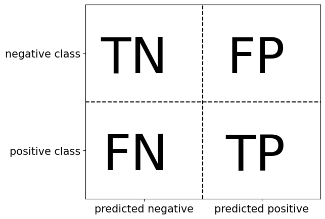
We can use the scikit-learn confusion_matrix() function to return the counts in the confusion matrix.
13.4.3 A closer look at the performance of the algorithms we ran on the digits data
13.4.3.1 Confusion Matrix for Logistic Regression Model
The confusion_matrix() method creates a 2-dimensional array of the confusion matrix numbers. It can be displayed as an array or plotted with the ConfusionMatrixDisplay object. Note that the ConfusionMatrixDisplay object also has from_predictions() and from_estimator() methods to plot the confusion matrix directly from the predictions and the true values, or from the estimator and the data. The methods for plotting from the predictions or from the estimator have more options. They can display counts, row percentages, column percentages, or overall percentages.
confusion = confusion_matrix(y_test, pred_logreg)
confusion
array([[402, 3],
[ 5, 40]])# We can plot a confusion matrix from the confusion matrix array
disp = ConfusionMatrixDisplay(confusion_matrix = confusion,
# display_labels = logreg.classes_)
display_labels = ['Not 9', '9'])
disp.plot()
plt.title('Confusion Matrix for Logistic Regression on Digits Data');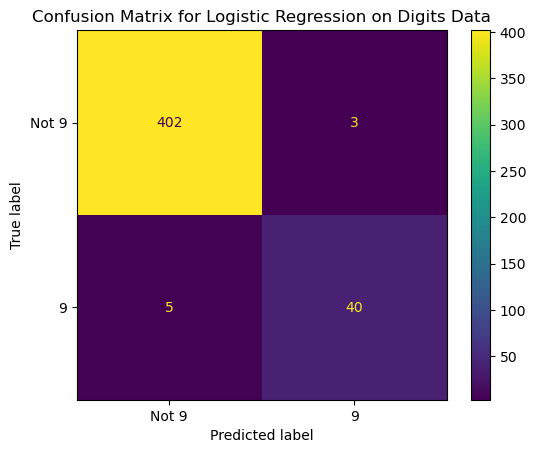
# We can also plot a confusion matrix from the predictions
# Note: Could add normalize = 'true' here to replace
# the counts with percentages (row-wise)
ConfusionMatrixDisplay.from_predictions(y_true = y_test,
                                        y_pred = pred_logreg ,
                                        display_labels = ['Not 9', '9'],
                                        # normalize = 'true',
                                        colorbar = False)

plt.title('Confusion Matrix for Logistic Regression on Digits Data');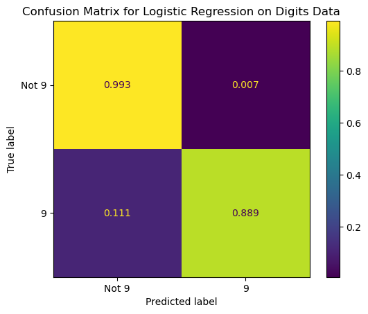
13.4.3.2 Confusion Matrix for Model that Predicts Most Frequent Class
ConfusionMatrixDisplay.from_predictions(y_true = y_test,
                                        y_pred = pred_most_frequent,
                                        display_labels = ['Not 9', '9'],
                                        # normalize = 'true',
                                        colorbar = False)

plt.title('Confusion Matrix for Predicting Most Frequent on Digits Data');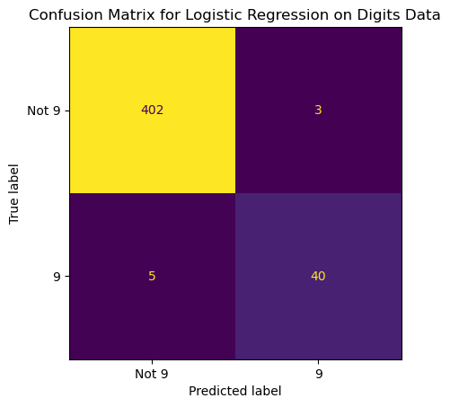
13.4.3.3 Confusion Matrix for Random Predictions According to the Training Set’s Class Distribution.
ConfusionMatrixDisplay.from_predictions(y_true = y_test,
                                        y_pred = pred_stratified,
                                        display_labels = ['Not 9', '9'],
                                        # normalize = 'true',
                                        colorbar = False)

plt.title('Confusion Matrix for Random Predictions on Digits Data');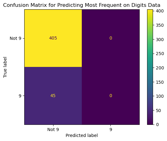
13.4.3.4 Confusion Matrix for Decision Tree Model
ConfusionMatrixDisplay.from_predictions(y_true = y_test,
                                        y_pred = pred_tree,
                                        display_labels = ['Not 9', '9'],
                                        # normalize = 'true',
                                        colorbar = False)

plt.title('Confusion Matrix for Decision Tree on Digits Data');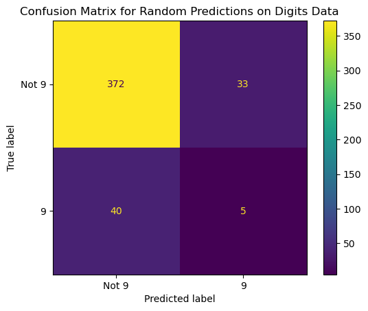
13.5 Metrics based on the confusion matrix
There are several metrics that can be calculated from the four components of the confusion matrix (TP, FP, TN, FN)
Simple Accuracy:
\(Accuracy = \frac{TP+TN}{TP+TN+FP+FN}\)
Precision, also known as positive predicted value (PPV), measures the percentage of samples predicted to be positive that are actually positive. It is used when it is important to limit the number of false positives.
\(Precision = \frac{TP}{TP+FP}\)
Recall, also called sensitivity, hit rate, and true positive rate (TPR), measures the percentage of samples that are actually positive that are predicted to be positive. Used when it is important to identify as many of the positive samples as possible, such as with a cancer test.
\(Recall = \frac{TP}{TP+FN}\)
The false positive rate (FPR) is the percentage samples that are actually negative that are predicted to be positive.
\(FPR = \frac{FP}{FP+TN}\)
There is a tradeoff between optimizing for precision and optimizing for recall. The f-score or f-measure is the harmonic mean of precision and recall. This particular variant of the f-measure is known as the \(f_1 score\).
\(F = 2 \times \frac{precision \times recall}{precision + recall}\)
13.5.0.1 Let’s calculate the \(f_1 score\) for the predictions we made earlier
Note how the \(f_1 score\) distinguishes between the models much better than simple accuracy.
print("f1 score most frequent: {:.2f}".format(
      f1_score(y_test, pred_most_frequent)))
print("f1 score predicting at random: {:.2f}".format(
      f1_score(y_test, pred_stratified)))
print("f1 score tree: {:.2f}".format(
      f1_score(y_test, pred_tree)))
print("f1 score logistic regression: {:.2f}".format(
      f1_score(y_test, pred_logreg)))
f1 score most frequent: 0.00
f1 score predicting at random: 0.04
f1 score tree: 0.76
f1 score logistic regression: 0.9113.5.1 The classification_report function gives us several metrics at once
print(classification_report(y_test, pred_tree,
                            target_names=["not nine", "nine"]))
precision recall f1-score support
not nine 0.97 0.97 0.97 405
nine 0.76 0.76 0.76 45
accuracy 0.95 450
macro avg 0.86 0.86 0.86 450
weighted avg 0.95 0.95 0.95 450
The classification_report function produces a set of metrics for each class as the positive class. support simply refers to the number of samples in each class. The macro avg is the simple average across classes. The weighted avg is the weighted average across the classes.
13.6 Taking uncertainty into account
The metrics we have seen so far are based on binary predictions, but most classification models can produce scores or probabilities via the decision_function() or predict_proba() methods. A binary class prediction can be understood as a combination of a score or probability and a threshold. In binary classification the threshold is typically set to 0 for the decision function and 0.5 for the predicted probability. The probabilities produced by classification models are not always very well calibrated, so we can sometimes improve performance on our metric of interest by adjusting the classification thresholds.
Let’s create some data and use a K-nn model do binary classification on the data.
X, y = make_blobs(n_samples=(4000, 500), cluster_std=[7.0, 2], random_state=22)

X_train, X_test, y_train, y_test = train_test_split(X, y, random_state=0)

knn = KNeighborsClassifier(n_neighbors = 35).fit(X_train, y_train)
See the probabilities of the positive class produced by the Knn model. 0.50 is the default probability threshold. Instances with probability of the positive class of 0.50 or higher will be classified as the positive class (1) and instances with probability of the positive class of less than 0.50 will be classified as the negative class (0).
knn.predict_proba(X_test)[:5]array([[1. , 0. ],
[0.28571429, 0.71428571],
[0.57142857, 0.42857143],
[1. , 0. ],
[1. , 0. ]])knn.predict(X_test)[:5]array([0, 1, 0, 0, 0])13.7 Making predictions at different thresholds
We can extract the probabilities of the positive class from the predict_proba() method and use them to make predictions at different thresholds. For example, in the cell below we use the np.where() function to make predictons on X_test at the 0.40 threshold. Notice that at the new threshold of 0.40 the third row, which we saw above has a probability of positive class of 0.4286, is now predicted to be positive class.
# Get second column (prob of positive class) from the predict_proba() method
prob_pos_class = knn.predict_proba(X_test)[:,1]

# Use np.where to make the predictions for 0.40 threshold
preds_40_thresh = np.where(prob_pos_class >= 0.40, 1, 0)

# View the first 5 rows of the predictions at the new threshold
preds_40_thresh[:5]
array([0, 1, 1, 0, 0])13.8 Receiver operating characteristics (ROC) and AUC
A popular tool for evaluating classifiers across all thresholds is the receiver operating characteristics curve or ROC curve. It displays the false positive rate (FPR) against the true positive rate (TPR). The roc_curve() function can be used to calculate the false positive rate and true positive rate at all the possible thresholds. The roc_curve() function takes as its inputs the actual target variable values and the probabilities of the positive class produced by the model.
fpr, tpr, thresholds = roc_curve(y_test, knn.predict_proba(X_test)[:,1])

plt.plot(fpr, tpr, label='ROC Curve')
plt.xlabel('FPR')
plt.ylabel('TPR (Recall)')

# Find threshold closest to 0.50
close_default = np.argmin(np.abs(thresholds - 0.5))

plt.plot(fpr[close_default], tpr[close_default], 'o', markersize=10, label='Threshold 0.5',
         fillstyle='none', c='k', mew=2)
plt.legend(loc=4)
plt.title('ROC Curve for K-nn Model');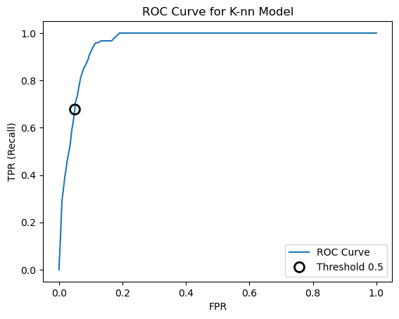
Let’s put the data from the plot into a DataFrame to try to better understand it.
roc_df_knn = pd.DataFrame({
    'Threshold': thresholds,
    'True Positive Rate': tpr,
    'False Positive Rate': fpr
})

roc_df_knn| Threshold | True Positive Rate | False Positive Rate | |
|---|---|---|---|
| 0 | inf | 0.000000 | 0.000000 |
| 1 | 0.828571 | 0.016529 | 0.000000 |
| 2 | 0.800000 | 0.066116 | 0.001992 |
| 3 | 0.771429 | 0.123967 | 0.003984 |
| 4 | 0.742857 | 0.289256 | 0.008964 |
| 5 | 0.714286 | 0.388430 | 0.017928 |
| 6 | 0.685714 | 0.454545 | 0.024900 |
| 7 | 0.657143 | 0.504132 | 0.031873 |
| 8 | 0.628571 | 0.537190 | 0.035857 |
| 9 | 0.600000 | 0.578512 | 0.038845 |
| 10 | 0.571429 | 0.636364 | 0.045817 |
| 11 | 0.542857 | 0.661157 | 0.047809 |
| 12 | 0.514286 | 0.677686 | 0.049801 |
| 13 | 0.485714 | 0.702479 | 0.050797 |
| 14 | 0.457143 | 0.735537 | 0.057769 |
| 15 | 0.428571 | 0.768595 | 0.061753 |
| 16 | 0.400000 | 0.809917 | 0.067729 |
| 17 | 0.371429 | 0.851240 | 0.077689 |
| 18 | 0.342857 | 0.867769 | 0.084661 |
| 19 | 0.314286 | 0.892562 | 0.092629 |
| 20 | 0.285714 | 0.900826 | 0.093625 |
| 21 | 0.257143 | 0.917355 | 0.098606 |
| 22 | 0.228571 | 0.942149 | 0.107570 |
| 23 | 0.200000 | 0.958678 | 0.115538 |
| 24 | 0.171429 | 0.958678 | 0.121514 |
| 25 | 0.142857 | 0.966942 | 0.132470 |
| 26 | 0.114286 | 0.966942 | 0.145418 |
| 27 | 0.085714 | 0.966942 | 0.165339 |
| 28 | 0.057143 | 1.000000 | 0.190239 |
| 29 | 0.028571 | 1.000000 | 0.245020 |
| 30 | 0.000000 | 1.000000 | 1.000000 |
13.8.1 Plot ROC curves for both K-nn and random forest classifiers
We can put the ROC curves for multiple prediction algorithms on the same plot to compare their performance.
rf = RandomForestClassifier()
rf.fit(X_train, y_train)

fpr_rf, tpr_rf, thresholds_rf = roc_curve(y_test, rf.predict_proba(X_test)[:, 1])

plt.plot(fpr, tpr, label='ROC Curve SVC')
plt.plot(fpr_rf, tpr_rf, label='ROC Curve RF')

plt.xlabel('FPR')
plt.ylabel('TPR (Recall)')
plt.plot(fpr[close_default], tpr[close_default], 'o', markersize=10, label='Threshold 0.5 K-nn',
         fillstyle='none', c='k', mew=2)

close_default_rf = np.argmin(np.abs(thresholds_rf - 0.5))

plt.plot(fpr_rf[close_default_rf], tpr_rf[close_default_rf], '^', markersize=10,
         label='Threshold 0.5 RF', fillstyle='none', c='k', mew=2)

plt.legend(loc=4)
plt.title('ROC Curves for K-nn and Random Forest Models');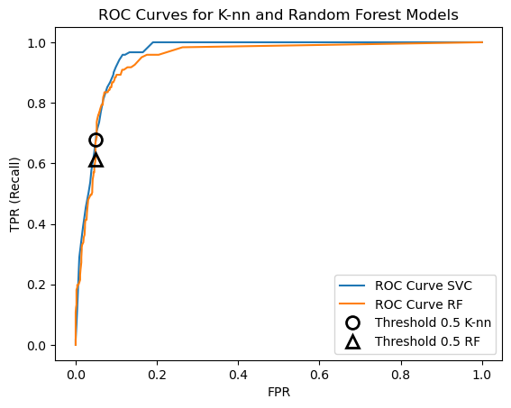
13.8.2 The area under the ROC curve is often used as a metric, called the AUC (“Area under ROC Curve”)
AUC is always between 0 and 1. Predicting randomly always produces an AUC with an expected value of 0.50. AUC is a better metric than simple accuracy for imbalanced classes. You can think of AUC as the probability that a randomly-selected point of the positive class will have a higher score (probability or ranking indicating likelihood of membership in the positive class) according to the classifier than a randomly-selected point of the negative class.
rf_auc = roc_auc_score(y_test, rf.predict_proba(X_test)[:, 1])
knn_auc = roc_auc_score(y_test, knn.predict_proba(X_test)[:, 1])
print('AUC for Random Forest: {:.3f}'.format(rf_auc))
print('AUC for Knn: {:.3f}'.format(knn_auc))
AUC for Random Forest: 0.946
AUC for Knn: 0.96013.8.3 A note about metrics for regression models
It is important to point out that all the metrics and tools we have discussed in this chapter apply only to classificatiom models. For regression models, in most cases the default metric \(R^2\) is sufficient. Sometimes mean squared error or mean absolute error is used instead.
13.9 Using metrics like AUC in model selection when using cross_validate() or GridSearchCV()
These have a scoring parameter that can be set to the metric you want to use.
13.9.1 With cross_validate()
You can specify the scoring metric tye cross_validate() function will use by setting the scoring parameter to one of a wide number of pre-defined strings, which can be listed with the get_scorer_names() function, or you can even define your own scoring function and use that.
all_scorers = get_scorer_names()
all_scorers
['accuracy',
'adjusted_mutual_info_score',
'adjusted_rand_score',
'average_precision',
'balanced_accuracy',
'completeness_score',
'd2_absolute_error_score',
'explained_variance',
'f1',
'f1_macro',
'f1_micro',
'f1_samples',
'f1_weighted',
'fowlkes_mallows_score',
'homogeneity_score',
'jaccard',
'jaccard_macro',
'jaccard_micro',
'jaccard_samples',
'jaccard_weighted',
'matthews_corrcoef',
'mutual_info_score',
'neg_brier_score',
'neg_log_loss',
'neg_max_error',
'neg_mean_absolute_error',
'neg_mean_absolute_percentage_error',
'neg_mean_gamma_deviance',
'neg_mean_poisson_deviance',
'neg_mean_squared_error',
'neg_mean_squared_log_error',
'neg_median_absolute_error',
'neg_negative_likelihood_ratio',
'neg_root_mean_squared_error',
'neg_root_mean_squared_log_error',
'normalized_mutual_info_score',
'positive_likelihood_ratio',
'precision',
'precision_macro',
'precision_micro',
'precision_samples',
'precision_weighted',
'r2',
'rand_score',
'recall',
'recall_macro',
'recall_micro',
'recall_samples',
'recall_weighted',
'roc_auc',
'roc_auc_ovo',
'roc_auc_ovo_weighted',
'roc_auc_ovr',
'roc_auc_ovr_weighted',
'top_k_accuracy',
'v_measure_score']# Load the digits dataset again
digits = load_digits()
y = digits.target == 9
X_train, X_test, y_train, y_test = train_test_split(digits.data, y, random_state = 57)# default scoring for classification is accuracy
result_acc = cross_validate(estimator = KNeighborsClassifier(n_neighbors = 35),
X = digits.data,
y = digits.target==9,
cv = 5)
print("Accuracy:", result_acc['test_score'].mean())Accuracy: 0.9760817084493965# Now let's try roc_auc score as the metric
result_roc = cross_validate(estimator = KNeighborsClassifier(n_neighbors = 35),
X = digits.data,
y = digits.target==9,
cv = 5,
scoring = 'roc_auc')
print("ROC AUC:", result_roc['test_score'].mean())ROC AUC: 0.994103579270131213.9.2 With the cross_validate() function we can also compute several metrics at once
res = cross_validate(estimator = KNeighborsClassifier(n_neighbors = 35),
                     X = digits.data,
                     y = digits.target==9,
                     cv = 5,
                     scoring=['accuracy', 'average_precision', 'recall_macro'])

pd.DataFrame(res)| fit_time | score_time | test_accuracy | test_average_precision | test_recall_macro | |
|---|---|---|---|---|---|
| 0 | 0.004656 | 0.028951 | 0.972222 | 0.939807 | 0.873457 |
| 1 | 0.001484 | 0.034118 | 0.961111 | 0.912051 | 0.830247 |
| 2 | 0.001673 | 0.032391 | 0.983287 | 0.983611 | 0.929008 |
| 3 | 0.001573 | 0.032725 | 0.988858 | 0.994133 | 0.944444 |
| 4 | 0.001386 | 0.090383 | 0.974930 | 0.952274 | 0.875000 |
13.9.3 We can also change the metric used to pick the best parameters in GridSearchCV()
This can result in different best parameters being found.
13.9.3.1 first use default metric, accuracy
param_grid = {'n_neighbors': range(1, 32, 2)}

gs = GridSearchCV(estimator = KNeighborsClassifier(),
                  param_grid = param_grid,
                  cv = RepeatedStratifiedKFold(n_splits = 10, n_repeats = 5))

gs.fit(X_train, y_train)
GridSearchCV(cv=RepeatedStratifiedKFold(n_repeats=5, n_splits=10, random_state=None),
estimator=KNeighborsClassifier(),
param_grid={'n_neighbors': range(1, 32, 2)})In a Jupyter environment, please rerun this cell to show the HTML representation or trust the notebook. On GitHub, the HTML representation is unable to render, please try loading this page with nbviewer.org.
Parameters
| estimator | KNeighborsClassifier() | |
| param_grid | {'n_neighbors': range(1, 32, 2)} | |
| scoring | None | |
| n_jobs | None | |
| refit | True | |
| cv | RepeatedStrat...om_state=None) | |
| verbose | 0 | |
| pre_dispatch | '2*n_jobs' | |
| error_score | nan | |
| return_train_score | False |
KNeighborsClassifier()
Parameters
| n_neighbors | 5 | |
| weights | 'uniform' | |
| algorithm | 'auto' | |
| leaf_size | 30 | |
| p | 2 | |
| metric | 'minkowski' | |
| metric_params | None | |
| n_jobs | None |
print("Grid search with accuracy")
print("Best parameters:", gs.best_params_)
print("Best cross validation score (accuracy): {:.3f}".format(gs.best_score_))
print("Test set accuracy: {:.3f}".format(accuracy_score(y_test, gs.predict(X_test))))
Grid search with accuracy
Best parameters: {'n_neighbors': 5}
Best cross validation score (accuracy): 0.996
Test set accuracy: 0.99113.9.3.2 Now use AUC as the metric instead of accuracy
grid = GridSearchCV(estimator = KNeighborsClassifier(),
                    param_grid = param_grid,
                    cv = RepeatedStratifiedKFold(n_splits = 10, n_repeats = 5),
                    scoring = 'roc_auc')

grid.fit(X_train, y_train)
GridSearchCV(cv=RepeatedStratifiedKFold(n_repeats=5, n_splits=10, random_state=None),
estimator=KNeighborsClassifier(),
param_grid={'n_neighbors': range(1, 32, 2)}, scoring='roc_auc')In a Jupyter environment, please rerun this cell to show the HTML representation or trust the notebook. On GitHub, the HTML representation is unable to render, please try loading this page with nbviewer.org.
Parameters
| estimator | KNeighborsClassifier() | |
| param_grid | {'n_neighbors': range(1, 32, 2)} | |
| scoring | 'roc_auc' | |
| n_jobs | None | |
| refit | True | |
| cv | RepeatedStrat...om_state=None) | |
| verbose | 0 | |
| pre_dispatch | '2*n_jobs' | |
| error_score | nan | |
| return_train_score | False |
KNeighborsClassifier(n_neighbors=11)
Parameters
| n_neighbors | 11 | |
| weights | 'uniform' | |
| algorithm | 'auto' | |
| leaf_size | 30 | |
| p | 2 | |
| metric | 'minkowski' | |
| metric_params | None | |
| n_jobs | None |
print("Grid search with AUC")
print("Best parameters:", grid.best_params_)
print("Best cross validation score (AUC): {:.3f}".format(grid.best_score_))
print("Test set accuracy: {:.3f}".format(accuracy_score(y_test, grid.predict(X_test))))
Grid search with AUC
Best parameters: {'n_neighbors': 11}
Best cross validation score (AUC): 0.994
Test set accuracy: 0.989