import time
import os
import numpy as np
import pandas as pd
from plotnine import *
import matplotlib.pyplot as plt

from sklearn.model_selection import train_test_split
from sklearn.model_selection import cross_validate
from sklearn.model_selection import RepeatedStratifiedKFold
from sklearn.model_selection import GridSearchCV

from sklearn.preprocessing import MinMaxScaler
from sklearn.preprocessing import StandardScaler
from sklearn.preprocessing import OneHotEncoder
from sklearn.preprocessing import PolynomialFeatures

from sklearn.compose import ColumnTransformer

from sklearn.pipeline import Pipeline

from sklearn.neighbors import KNeighborsClassifier
from sklearn.linear_model import LogisticRegression10 Model Building for Supervised Machine Learning
Click here to download this chapter as a Jupyter (.ipynb) file.
This chapter explains and demonstrates how the following tasks can be structured to build a supervised machine learning model, using scikit-learn tools:
- Proprocessing - Getting the data ready for the specific machine-learning algorithms that will be tried
- Estimating generalization performance - Estimating how each machine-learning algorithm will perform on new data that was not used to train it. This is also called performance on out-of-sample data
- Model tuning - Determining the best parameter setting(s) for each machine-learning algorithm
The chapter culminates with explanation and demonstration of how to accomplish both model tuning and estimation of generalization performance. They can’t be accomplished at the same time without biasing the estimate of generalization performance, so we will learn how to first estimate generalization performance for one or more algorithms, and then determine the best parameter settings for the model with the best estimated generalization performance.
10.1 Module and Function Imports
10.2 Load the Titanic Data
In this chapter we will again be using the Titanic data, which describes passengers on the Titanic. Below is a brief description of the variables:
Survived- the target variable. Has values 0 or 1, with 1 representing that the passenger survived the disasterSibSp- represents number of siblings or spouse traveling with the passengerParch- represents the number of parents or children traveling with the passengerPclass- represents class of ticketEmbarked- represents the port from which the passenger embarked.
Note: This is only a subset of the actual Titanic dataset.
titanic = pd.read_csv('https://neuronjolt.com/data/titanic.csv')titanic.info()<class 'pandas.core.frame.DataFrame'>
RangeIndex: 712 entries, 0 to 711
Data columns (total 7 columns):
# Column Non-Null Count Dtype
--- ------ -------------- -----
0 Survived 712 non-null int64
1 Pclass 712 non-null int64
2 Sex 712 non-null object
3 Age 712 non-null float64
4 SibSp 712 non-null int64
5 Parch 712 non-null int64
6 Embarked 712 non-null object
dtypes: float64(1), int64(4), object(2)
memory usage: 39.1+ KBfeatures = titanic.drop(columns = 'Survived')
target = titanic['Survived']10.3 Estimating Generalization Performance with Cross Validation
The purpose of supervised machine learning is to build a model that can effectively predict the values of a target variable based on the values of a set of other variables called the features. We use labeled training data to build the model, but as we do so we want to build the model that will make the best predictions for new, unlabeled data in the future. This is called generalization performance or out-of-sample performance.
We typically estimate generalization performance by splitting our labeled data into two parts, the training set and the test set. We build the model on the training set, with no participation whatsoever from the test set, and then we pretend that the test set is new unlabeled data for which we need to make predictions. We make the predictions, and then we estimate generalization performance by comparing the predictions to the actual values of the target variable.
To prevent our estimate of generalization performance from being overly influenced by the random features of one train-test split we typically split the data multiple times, giving us several test-set performances. The mean of several test set performance is a more reliable estimate of generalization performance than performance on a single test set. The term for this process of repeatedly dividing our data into training and test data for the purpose of estimating generalization performance is cross validation. In this section we will learn about several methods for cross validation.
10.3.1 K-Fold Cross Validation
K-fold cross validation is the most commonly-used form of cross validation. In k-fold cross validation the data is divided randomly into \(k\) parts of approximately equal size, called folds. Next, a sequence of \(k\) models is trained and tested, with each fold taking a turn serving as the test data. Usually the first \(\frac{1}{k}\) of the data serves as the first fold, and so on.
For example, to implement 5-fold cross validation you would first divide the data into 5 folds, then do 5 splits. Each of the 5 folds serves as the test data for one of the splits, with the other folds serving as the training data for that split. The diagram below demonstrates 5-fold cross validation.
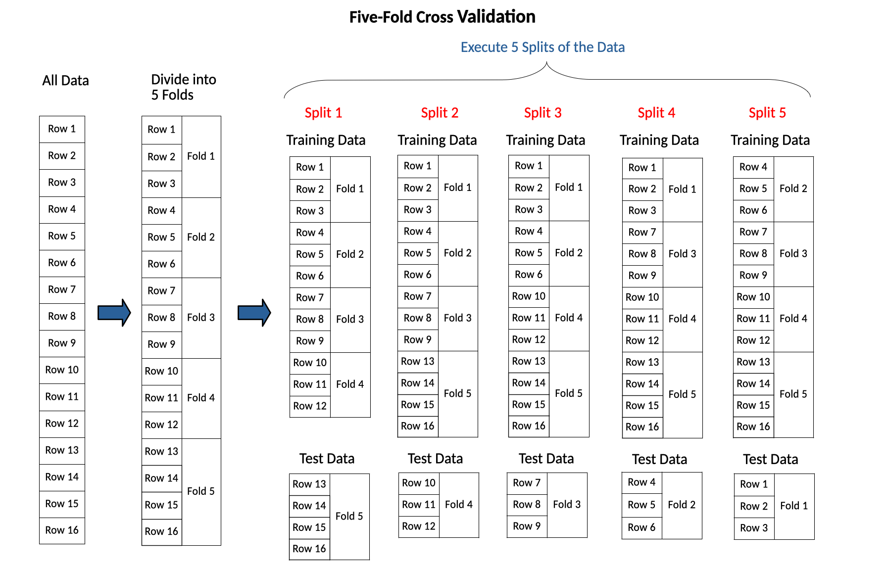
K-fold cross validation uses the labeled data more efficiently than multiple random train-test splits. With K-fold cross validation each row is treated equally; each row is in the test set \(k\) times and in the training set \(k-1\) times. This is an improvement over multiple random train-test splits, because with multiple random train-test splits one row might be overrepresented in the test sets while another row is overrepresented in the training sets.
K-fold cross validation is the default form of cross validation used by scikit-learn’s cross_validate() function (used to estimate generalization performance) and GridSearchCV() function (used for model tuning with grid search, which we will see in a later section of this chapter). Those functions use K-fold cross validation when the target is numeric and stratified K-fold cross validation when the target is categorical. The term stratified means that when the data is divided into folds the function attempts to keep the ratio of values of the target class the same in each fold. For example, if we are building a model to predict whether a cell is cancerous or not and 45% of the rows overall are cancerous, the splitting procedure for stratified K-fold cross validation attempts to split the data so that the percentage of cancerous rows in each fold is as close to 45% as possible.
10.3.2 Define a Splitter to use other types of cross validation
If you want to use a cross validation strategy other than K-fold or stratified K-fold, or if you want to override the default parameters for K-fold or stratified K-fold cross validation you can use a scikit-learn splitter object to define and implement the cross validation strategy. Splitter objects implement a specific type of splitting strategy for cross validation. They are created with constructor functions similar to how estimators or transformers are created. Examples of the splitters available in scikit-learn include the following:
- K-fold cross validation (create with
KFold()function) - divide the data into k folds; each fold takes a turn as the test fold, with the other folds used for training. When using the splitter object for K-fold you can instruct it to shuffle the data first. This is the default splitter for thecross_validate()function for regression tasks. Note that K-fold cross validation in scikit-learn doesn’t shuffle the samples by default before creating the folds. This could lead to problems if the data is sorted in some systematic fashion. TheKFold()splitter function has ashuffleparameter that can be set toTrueto shuffle the data before the folds are defined - Stratified K-fold cross validation (create with
StratifiedKFold()function) - like k-fold cross validation, but the splits maintain the relative proportions of the target class values in each fold. This is the default splitter for thecross_validate()function for classification tasks. - Repeated K-fold cross validation (create with
RepeatedKFold()function) - perform k-fold more than once, shuffling the data in between - Repeated Stratified K-fold cross validation (create with
RepeatedStratifiedKFold()function) - like repeated K-fold, but stratified - Leave-one-out cross validation (create with
LeaveOneOut()function) - each fold is a single instance - Shuffle-split cross validation (create with
ShuffleSplit()function) - like random train-test splitting, specifying either number of instances in train and test, or percentage of dataset in train and test. Use for regression tasks. - Stratified shuffle-split cross validation (create with
StratifiedShuffleSplit()function) - use for classification tasks. - GroupKFold (create with
GroupKFold()function) - takes a groups array parameter to indicate groups in the data that should not be split when creating the training and test sets. For example, if you have medical data where you have multiple samples from the same patient but want to train models to generalize to new patients you can specify the patients as groups and prevent them from being split across training and testing data. Another example would be when you are training a speech recognition model and have multiple speech recordings from the same speaker but want to train a model to recognize speech of new speakers.
Note that instances of these Splitter classes may be passed to the cross_validate(), or GridSearchCV() functions via the cv parameter.
10.3.3 Example of K-fold cross validation
Scikit-learn provides the cross_validate() function to do cross validation. It uses 5-fold cross validation by default for regression tasks and stratified 5-fold cross validation by default for classification tasks. It also has a cv parameter that may be used to specify a different splitting strategy.
As an example of how to use K-fold cross validation to estimate the generalization performance of a particular model we will use the cross_validate() function to estimate how well a 10-nearest neighbor model performs on the Titanic data. The Titanic data has both numeric and categorical features, so we will need to min-max scale the numeric features and one-hot encode the categorical features.
10.3.4 Combining steps with a scikit-learn Pipeline
To perform the cross validation of the 10-nearest neighbor model on the Titanic data requires several train-test splits. The data will need to be preprocessed and the model trained and tested after every split. Scikit-learn provides a class called a Pipeline that we can use to combine steps such as preprocessing and estimating. A pipeline, created with the Pipeline() constructor function, allows us to sequentially apply a list of transformers to preprocess the data and, if desired, conclude the sequence with a estimator. All the intermediate steps of the pipeline must be be transformers, that is, they must be objects that implement fit() and transform() methods. If an estimator is added as the final step in the pipeline it only needs to implement the fit() method. Conveniently, if the final step of a pipeline is an estimator the pipeline itself functions as an estimator and has the usual fit(), predict() and score() methods. It may be used as the estimator parameter in a cross_validate() function or any other function that requires an estimator.
The purpose of a pipeline is to assemble several steps that can be cross-validated together. When a preprocessing step is combined with an estimator in a pipeline scikit-learn ensures that the preprocessing is done correctly; that is, at each split transformations such as scaling are always fit to the training data first and then used to transform both the training and test data.
Below we create a column transformer that may be used to min-max scale numeric features and one-hot encode categorical features. Then, we combine that column transformer with the estimator, 10-nearest neighbors, in a pipeline.
# Create a column transformer
ct = ColumnTransformer([
    ('min_max', MinMaxScaler(), ['Age', 'SibSp', 'Parch']),
    ('one_hot', OneHotEncoder(), ['Pclass', 'Sex', 'Embarked'])
])
# Package the column transformer together with the 10-nn model in a pipeline
knn_pipe = Pipeline([
('preprocessing', ct),
('classification', KNeighborsClassifier(n_neighbors = 10))
])Next we use the cross_validate() function to estimate generalization performance of the 10-nearest neighbor model on the Titanic data. The cross validation strategy defaults to 5-fold cross validation. A different strategy may be defined by using the cv parameter. When the cv parameter is set to an integer that integer becomes the number of folds to be used in K-fold or stratified K-fold cross validation. It may also be set to a splitter object if we used a splitter object to define a different splitting strategy. Below we set cv = 10 to specify 10-fold cross validation. Stratified 10-fold cross validation will be used because the target variable is categorical.
The cross_validate() function returns a dictionary containing training and scoring times, the test score, and optionally the training score for each split. The dictionary returned is easily converted to a pandas DataFrame for display or analysis.
scores = cross_validate(estimator = knn_pipe,
                         X = features,
                         y = target,
                         cv = 10)
# View the scores dictionary
scores{'fit_time': array([0.018996 , 0.01113081, 0.00938892, 0.00882006, 0.00891328,
0.00871801, 0.00867105, 0.00853205, 0.00911903, 0.00850415]),
'score_time': array([0.00847006, 0.00714898, 0.0072279 , 0.00863791, 0.0073719 ,
0.00703597, 0.00711393, 0.00700593, 0.00686407, 0.00690985]),
'test_score': array([0.72222222, 0.76388889, 0.8028169 , 0.74647887, 0.84507042,
0.74647887, 0.85915493, 0.78873239, 0.73239437, 0.88732394])}# Convert the scores dictionary to a pandas DataFrame and view it
scores_df = pd.DataFrame(scores)
scores_df| fit_time | score_time | test_score | |
|---|---|---|---|
| 0 | 0.018996 | 0.008470 | 0.722222 |
| 1 | 0.011131 | 0.007149 | 0.763889 |
| 2 | 0.009389 | 0.007228 | 0.802817 |
| 3 | 0.008820 | 0.008638 | 0.746479 |
| 4 | 0.008913 | 0.007372 | 0.845070 |
| 5 | 0.008718 | 0.007036 | 0.746479 |
| 6 | 0.008671 | 0.007114 | 0.859155 |
| 7 | 0.008532 | 0.007006 | 0.788732 |
| 8 | 0.009119 | 0.006864 | 0.732394 |
| 9 | 0.008504 | 0.006910 | 0.887324 |
Note how the test score (accuracy on predictions on the test fold) varies between the train-test splits. The Titanic data only has 712 rows, so it is a good example of a small dataset for which the mean of test performance over multiple splits should be used to estimate generalization performance.
Below we calculate the mean test score across the splits as our estimate of generalization performance of the 10-nn model on the Titanic data.
# Calculate the mean of the test_score column, which is our
# estimate of generalization performance
scores_df['test_score'].mean()np.float64(0.7894561815336464)10.4 Model Tuning with Grid Search
Model Tuning is the general term for the process of finding the parameter settings for the underlying prediction algorithm that result in the best estimated generalization performance. Other names for this process are Parameter Tuning and Hyperparameter Tuning. Grid Search is a common technique used for model tuning. Grid search refers to the process of estimating out-of-sample performance for an algorithm for a set of different parameter settings in order to find the parameter setting at which the model performs best on the data. Grid search uses cross validation internally. At each split of the cross validation, models using each of the parameter settings are built on the training data and scored on the test data. In this way, each parameter combination will have several test performances which may then be averaged to obtain a robust estimate of the model’s generalization performance with that particular parameter setting.
We actually performed a grid search in Chapter 7, when we generated the data for a validation curve graph for the K-nn model. We used nested looping code, with data splitting in the outer loop and training and testing for all values of \(k\) in the inner loop. In this chapter we will use the scikit-learn GridSearchCV() function to perform grid search rather than constructing our own nested looping code.
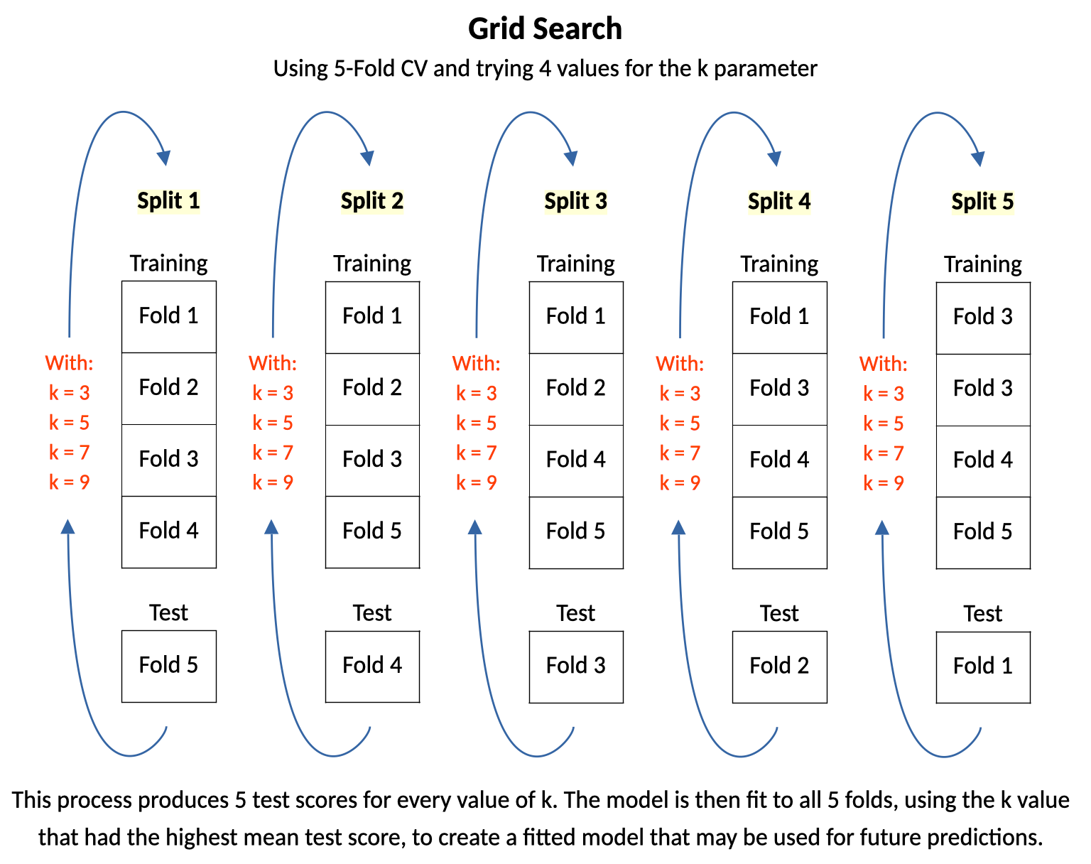
The diagram below illustrates a grid search that uses 5-fold cross validation and tries 4 different settings for k in a K-nn model. At each split, models for each k parameter setting are trained on the training folds and tested on the test fold. When this process completes there are 5 test scores for each value of the k parameter. In its final step the grid search fits a model to all 5 folds, using the k parameter value that had the highest mean test score.
10.4.1 Accomplishing Both Model Tuning and Estimation of Generalization Performance
10.4.1.1 Another Level of Splitting is Needed
The purpose of a grid search is to find the best parameter setting(s) for an algorithm. After the cross validation within the grid search completes, the mean test performance across the splits for each parameter setting is calculated. The setting with the highest mean test performance is the best parameter setting. The grid search will then train the algorithm again, at its best parameter setting, on all the data.
It is important to note, however, that the mean test performance across the splits should not be used as an estimate of generalization performance. It should only be used to determine the best parameter setting(s) for the model. The reason it should not be used as an estimate of generalization performance is because the same test data is used multiple times across different parameter settings. This reuse introduces bias because the model selection process implicitly tailors the parameters to the test data, which likely gives performance estimates for those parameters an optimistic bias.
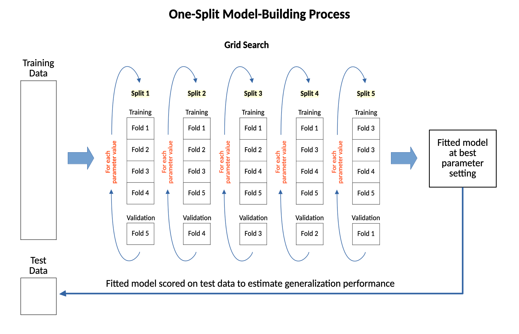
To combine model tuning with estimation of generalization performance another level of data splitting is added. The data is first split into training data and test data. The training data is used for model tuning and the test data is used to estimate generalization performance. As part of the model tuning process the training data from the first level of splitting gets repeatedly split into training data and validation data by the grid search that tests the algorithm at each parameter setting. Once the best parameter setting is found the grid search then trains the algorithm at its best parameter setting on all the training data from the original split. After it does this, the grid search is then ready to make predictions on future data. We then score the grid search on the test data from the outer-level split to estimate its generalization performance.
This model-building process bases its estimate of generalization performance on just one train-test split. This is an appropriate approach to model building only if we have a large amount of data.
The diagram below shows this one-split model-building process. All the data is split one time into training data and test data. Then, a full grid search is run on the training data to find the best parameter setting and fit the model at that best parameter setting to all the training data. The grid search is then scored on the test data to provide the estimate of generalization performance.
10.5 One-Split Model Building Process with Logistic Regression on the Titanic Data
In this section we will practice the basic model-building process, where we base our estimate of generalization performance on only one train-test split. We will do a train-test split of the Titanic data, conduct a grid search on the training data with a logistic regression algorithm, and then use the fitted grid search object to score the model on the test data. This score is our estimate of generalization performance for logistic regression on this data. We typically use this model-building approach to estimate generalization performance for several predictive algorithms. Then, the final step in the modeling process is to re-run the grid search for the best-performing algorithm on ALL the data to tune the model and prepare it to make predictions on future data. This process is a full model building process that can work well if you have a lot of data. If you don’t have a lot of data this process is not recommended because it bases its estimate of generalization performance on just one train-test split.
Logistic regression is a form of linear regression that is used to make predictions when the target is categorical. It has a parameter, C, that controls the model’s flexibility to fit the training data. The higher C is, the more flexible the model is to fit the training data. We will use the GridSearchCV() function to create the GridSearch object.
10.5.1 Split the Titanic data into training and test sets
Split the Titanic data into training and test sets. Use a stratified split, since the target variable is categorical.
X_train, X_test, y_train, y_test = train_test_split(features,
                                                    target,
                                                    stratify = target)
10.5.2 Define lists for the categorical and numeric features
We can then use these lists in our column transformer, rather than having to list out the specific features for each step.
cat_features = ['Sex', 'Pclass', 'Embarked']
num_features = ['Age', 'SibSp', 'Parch']
10.5.3 Combine the pre-processing and estimation steps in a pipeline
In the code cells below we create a column transformer for the Titanic data and then package the column transformer together with the logistic regression estimator in a pipeline. In the column transformer we will one-hot encode the categorical features. We will try doing two things to the numeric features. First we will apply the PolynomialFeatures() function out to degree 3 to add squared features, cubed features, and interactions, and then we will standard-scale the resulting numeric features. Because we are doing two things to the numeric features - adding polynomial features and then standard scaling - we will package those two things into a pipeline.
We add the interaction terms and polynomial features to give the model more flexibility to fit the training data. This will help prevent it from underfitting. We don’t need to worry too much about overfitting, because the C parameter for logistic regression gives us a tool to use to make fine-grained changes in the flexibility level of the algorithm, and the grid search will help us to set the C parameter to the right level. This is a common pre-processing approach that we will learn more about in the next chapter.
ct = ColumnTransformer([
    ('poly_std', Pipeline([('poly', PolynomialFeatures(degree = 3, include_bias = False)),
                            ('std', StandardScaler())]), num_features),
    ('one_hot', OneHotEncoder(handle_unknown = 'ignore'), cat_features)
])
pipe = Pipeline([
('pre', ct),
('cls', LogisticRegression(max_iter = 2_000))
])10.5.4 Specify the parameter values to try
The pipeline we created can serve as the estimator in the GridSearchCV() function because its last step is an estimator. When we specify the values of parameter C that we want to try we need to specify them in a way that provides the information needed to pass the parameters to the correct step of the pipeline. To do so, we need to specify the parameters in a dictionary and use the following convention for the key value in the dictionary:
the step in the pipeline, followed by two underscores, followed by the parameter name.
The parameter C is the parameter for logistic regression that influences the model’s flexibility to fit the training data. The higher C is the more flexible the model is to fit the training data. It should be varied on a logarithmic scale.
Below we set up a parameter grid to test various settings of the C parameter, generating 16 values on a logarithmic scale between \(10^{-4}\) and \(10^4\), or between 0.0001 and 10,000.
How do we know what range to use for the parameter setting? Although experience can eventually provide you with good starting points for various parameter settings, the short answer is that we don’t know before running the grid search what the best parameter setting will be, so we typically set the parameter to a fairly wide range and try the grid search. Then we examine the results of the grid search to see if we need to adjust the parameter setting values. If the best parameter setting, for example, was at either end of the range of parameter settings we tried, we would need to widen the range for the parameter setting to make sure we find the true best parameter setting, not just the best one of the set we tried. The best way to determine if the range of parameter settings we tried includes the best parameter setting or not is to make a validation curve plot. If our range for the parameter is wide enough we should see that the test performance curve has a peak, with areas of lower performance on either side of the peak.
Another use of the validation curve plot is that it can show us the range of the parameter setting at which performance is near peak. We can then re-run the grid search with the parameter range focused on that range.
pgrid = {
    'cls__C': np.logspace(-4, 4, 16)
}
10.5.5 Instantiate an object of the GridSearchCV class
Specify the estimator, the parameter grid to search, and the cross validation strategy. The cross validation will be performed for every parameter combination from the parameter grid. Here we use 6-fold cross validation. It will be stratified by default, because the target variable in the Titanic data is categorical.
Note that we also retain the scores on the training data so that we can make a validation curve plot, and we set the scoring metric to ‘accuracy’. This is the default performance metric, but in a later chapter we will learn about other metrics that can be used instead.
grid_search = GridSearchCV(estimator = pipe,
                           param_grid = pgrid,
                           cv = 6,
                           scoring = 'accuracy',
                           return_train_score = True)
10.5.6 Do an initial fit of the grid search to the training data
The fit() method of GridSearchCV finds the best parameters through a cross validation process in which at each split a model is built and tested for every value of the parameter setting. The best parameter setting is the one that has the highest mean performance on the test folds. After the best parameter setting is identified the grid search automatically fits a model with the best parameter settings to the whole training set. The fitted GridSearchCV object is thus itself an estimator, with fit(), predict(), and score() methods.
grid_search.fit(X_train, y_train)GridSearchCV(cv=6,
estimator=Pipeline(steps=[('pre',
ColumnTransformer(transformers=[('poly_std',
Pipeline(steps=[('poly',
PolynomialFeatures(degree=3,
include_bias=False)),
('std',
StandardScaler())]),
['Age',
'SibSp',
'Parch']),
('one_hot',
OneHotEncoder(handle_unknown='ignore'),
['Sex',
'Pclass',
'Embarked'])])),
('cls',
LogisticRegression(max_iter=2000))]),
param_grid={'cls__C': array([1.00000000e-04, 3.41454887e-04, 1.16591440e-03, 3.98107171e-03,
1.35935639e-02, 4.64158883e-02, 1.58489319e-01, 5.41169527e-01,
1.84784980e+00, 6.30957344e+00, 2.15443469e+01, 7.35642254e+01,
2.51188643e+02, 8.57695899e+02, 2.92864456e+03, 1.00000000e+04])},
return_train_score=True, scoring='accuracy')In a Jupyter environment, please rerun this cell to show the HTML representation or trust the notebook. On GitHub, the HTML representation is unable to render, please try loading this page with nbviewer.org.
Parameters
| estimator | Pipeline(step..._iter=2000))]) | |
| param_grid | {'cls__C': array([1.0000...00000000e+04])} | |
| scoring | 'accuracy' | |
| n_jobs | None | |
| refit | True | |
| cv | 6 | |
| verbose | 0 | |
| pre_dispatch | '2*n_jobs' | |
| error_score | nan | |
| return_train_score | True |
Parameters
| transformers | [('poly_std', ...), ('one_hot', ...)] | |
| remainder | 'drop' | |
| sparse_threshold | 0.3 | |
| n_jobs | None | |
| transformer_weights | None | |
| verbose | False | |
| verbose_feature_names_out | True | |
| force_int_remainder_cols | 'deprecated' |
['Age', 'SibSp', 'Parch']
Parameters
| degree | 3 | |
| interaction_only | False | |
| include_bias | False | |
| order | 'C' |
Parameters
| copy | True | |
| with_mean | True | |
| with_std | True |
['Sex', 'Pclass', 'Embarked']
Parameters
| categories | 'auto' | |
| drop | None | |
| sparse_output | True | |
| dtype | <class 'numpy.float64'> | |
| handle_unknown | 'ignore' | |
| min_frequency | None | |
| max_categories | None | |
| feature_name_combiner | 'concat' |
Parameters
| penalty | 'l2' | |
| dual | False | |
| tol | 0.0001 | |
| C | np.float64(0....8931924611143) | |
| fit_intercept | True | |
| intercept_scaling | 1 | |
| class_weight | None | |
| random_state | None | |
| solver | 'lbfgs' | |
| max_iter | 2000 | |
| multi_class | 'deprecated' | |
| verbose | 0 | |
| warm_start | False | |
| n_jobs | None | |
| l1_ratio | None |
10.5.7 View the pattern of test performance vs parameter setting
It is important to check the best parameter setting after the grid search and compare it to the range of values you specified for the parameter. If the best parameter setting is at or very near the ends of the ranges of values you specified in your parameter grid for the grid search you should widen the parameter grid and re-run the grid search.
Conversely, if the best parameter setting is in the middle of the range of values you specified for your parameter grid you might want to narrow the range and re-run the grid search.
Below we will view the best parameter setting and also make a validation curve plot to see the pattern of test performance vs the parameter settings.
# Best parameter setting from the grid search
grid_search.best_params_
{'cls__C': np.float64(0.15848931924611143)}To make the validation curve plot we first need to put the relevant grid search results into a DataFrame and then melt it to long format so we can show both training and test performance on the same plot. The grid search results are stored in a dictionary accessed with the grid search’s cv_results_ property. This results dictionary can be easily converted to a pandas DataFrame for viewing and analysis.
gs_results_df = pd.DataFrame(grid_search.cv_results_)
gs_results_df.columns
Index(['mean_fit_time', 'std_fit_time', 'mean_score_time', 'std_score_time',
'param_cls__C', 'params', 'split0_test_score', 'split1_test_score',
'split2_test_score', 'split3_test_score', 'split4_test_score',
'split5_test_score', 'mean_test_score', 'std_test_score',
'rank_test_score', 'split0_train_score', 'split1_train_score',
'split2_train_score', 'split3_train_score', 'split4_train_score',
'split5_train_score', 'mean_train_score', 'std_train_score'],
dtype='object')vc_plot_data = gs_results_df.loc[:, ['param_cls__C', 'mean_test_score', 'mean_train_score']]
vc_plot_data_long = vc_plot_data.melt(id_vars = 'param_cls__C',
var_name = 'perf_type',
value_name = 'accuracy')
vc_plot_data_long.sample(5)| param_cls__C | perf_type | accuracy | |
|---|---|---|---|
| 27 | 73.564225 | mean_train_score | 0.822472 |
| 29 | 857.695899 | mean_train_score | 0.821348 |
| 2 | 0.001166 | mean_test_score | 0.595506 |
| 30 | 2928.644565 | mean_train_score | 0.820974 |
| 8 | 1.847850 | mean_test_score | 0.792135 |
# Create the validation curve plot with plotnine
(
    ggplot(data = vc_plot_data_long, mapping = aes(x = 'param_cls__C', y = 'accuracy', color = 'perf_type'))
    + geom_line(size = 1)
    + geom_hline(yintercept = vc_plot_data.iloc[vc_plot_data['mean_test_score'].idxmax()]['mean_test_score'],
                 linetype = ':', size = 1)
    + scale_x_log10()
    + theme_light()
    + labs(title = "Validation Curve Plot for Logistic Regression",
           x = "C Parameter",
           y = "Accuracy")
)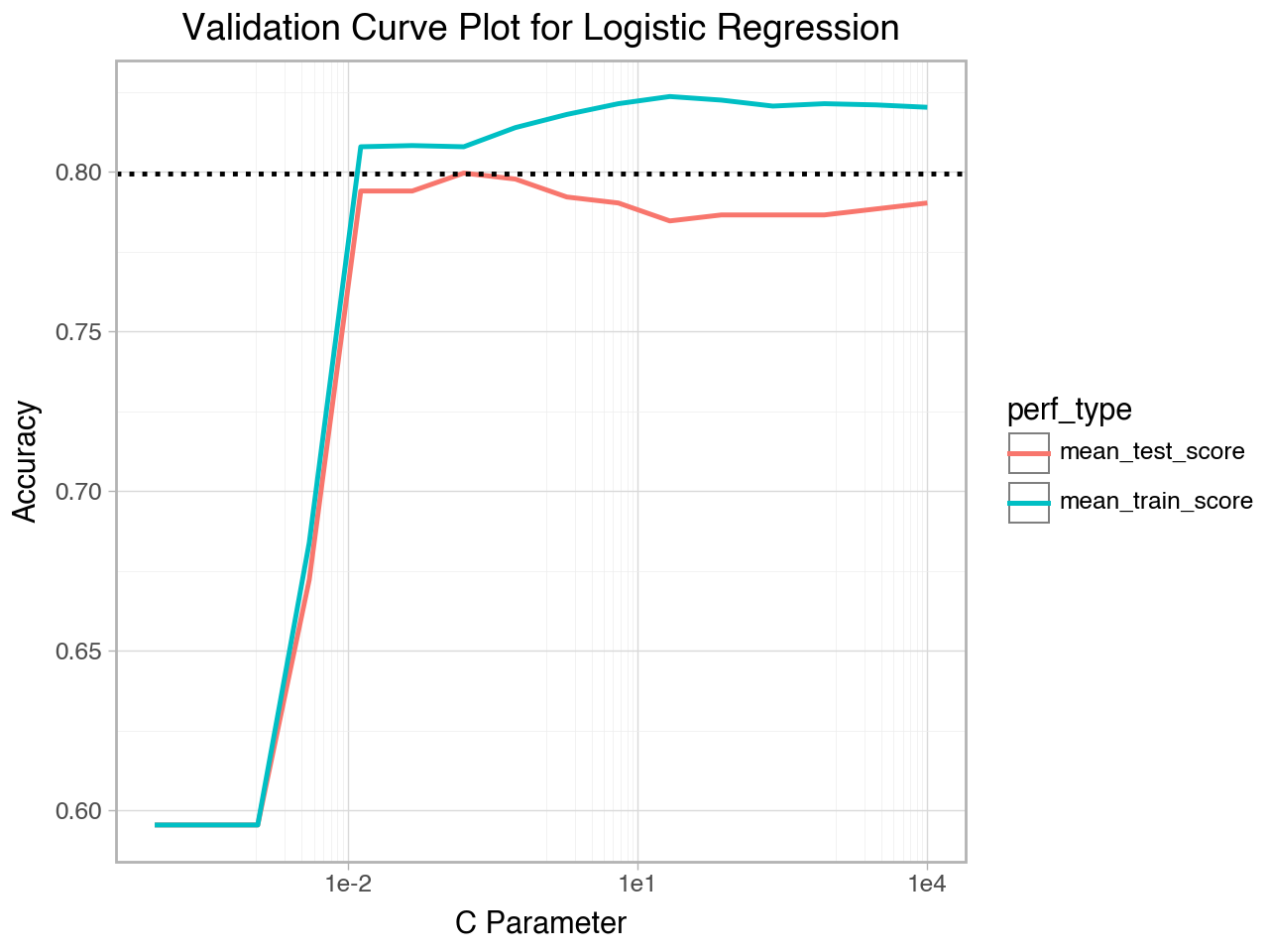
10.5.8 Redefine the parameter grid and then re-run the grid search
Since the best parameter setting is between \(10^{-3}\) and \(10^1\) let’s redefine the parameter grid to that range and include more parameter candidates so that they are closer together, then re-run the grid search. This will give us a better chance of getting the grid search set to the true best parameter setting.
# re-define the parameter settings, based on what we saw in the
# validation curve plot
pgrid = {
    'cls__C': np.logspace(-3, 1, 24)
}

# re-define the grid search
grid_search = GridSearchCV(estimator = pipe,
                           param_grid = pgrid,
                           cv = 6,
                           scoring = 'accuracy',
                           return_train_score = True)

# fit the grid search to the training data
grid_search.fit(X_train, y_train)
GridSearchCV(cv=6,
estimator=Pipeline(steps=[('pre',
ColumnTransformer(transformers=[('poly_std',
Pipeline(steps=[('poly',
PolynomialFeatures(degree=3,
include_bias=False)),
('std',
StandardScaler())]),
['Age',
'SibSp',
'Parch']),
('one_hot',
OneHotEncoder(handle_unknown='ignore'),
['Sex',
'Pclass',
'Embarked'])])),
('cls',
LogisticRegression(max_iter=2000))]),
para...-03,
4.96194760e-03, 7.40568469e-03, 1.10529514e-02, 1.64964807e-02,
2.46209240e-02, 3.67466194e-02, 5.48441658e-02, 8.18546731e-02,
1.22167735e-01, 1.82334800e-01, 2.72133877e-01, 4.06158599e-01,
6.06189899e-01, 9.04735724e-01, 1.35031404e+00, 2.01533769e+00,
3.00788252e+00, 4.48925126e+00, 6.70018750e+00, 1.00000000e+01])},
return_train_score=True, scoring='accuracy')In a Jupyter environment, please rerun this cell to show the HTML representation or trust the notebook. On GitHub, the HTML representation is unable to render, please try loading this page with nbviewer.org.
Parameters
| estimator | Pipeline(step..._iter=2000))]) | |
| param_grid | {'cls__C': array([1.0000...00000000e+01])} | |
| scoring | 'accuracy' | |
| n_jobs | None | |
| refit | True | |
| cv | 6 | |
| verbose | 0 | |
| pre_dispatch | '2*n_jobs' | |
| error_score | nan | |
| return_train_score | True |
Parameters
| transformers | [('poly_std', ...), ('one_hot', ...)] | |
| remainder | 'drop' | |
| sparse_threshold | 0.3 | |
| n_jobs | None | |
| transformer_weights | None | |
| verbose | False | |
| verbose_feature_names_out | True | |
| force_int_remainder_cols | 'deprecated' |
['Age', 'SibSp', 'Parch']
Parameters
| degree | 3 | |
| interaction_only | False | |
| include_bias | False | |
| order | 'C' |
Parameters
| copy | True | |
| with_mean | True | |
| with_std | True |
['Sex', 'Pclass', 'Embarked']
Parameters
| categories | 'auto' | |
| drop | None | |
| sparse_output | True | |
| dtype | <class 'numpy.float64'> | |
| handle_unknown | 'ignore' | |
| min_frequency | None | |
| max_categories | None | |
| feature_name_combiner | 'concat' |
Parameters
| penalty | 'l2' | |
| dual | False | |
| tol | 0.0001 | |
| C | np.float64(0.6061898993497572) | |
| fit_intercept | True | |
| intercept_scaling | 1 | |
| class_weight | None | |
| random_state | None | |
| solver | 'lbfgs' | |
| max_iter | 2000 | |
| multi_class | 'deprecated' | |
| verbose | 0 | |
| warm_start | False | |
| n_jobs | None | |
| l1_ratio | None |
# View the best parameter setting from the grid search
grid_search.best_params_
{'cls__C': np.float64(0.6061898993497572)}10.5.9 Score the grid search on the test data to estimate generalization performance
This is the test data from the original train-test split. The training data from the original split was used in the grid search to find the best parameter setting. Now we can use the test data to estimate the model’s generalization performance, since it wasn’t used to set the parameters.
grid_search.score(X_test, y_test)0.792134831460674210.5.10 Perform a second grid search on all the data to tune the final model and prepare for future predictions
In a typical model-building process we would go through this process for several predictive algorithms in order to find the one with the best estimated generalization performance. Then, for the algorithm with the best estimated generalization performance we would perform a final tuning of the model by re-running the grid search on all the data. After this grid search object is fit to all the data it may be used as an estimator to make predictions for future data.
grid_search.fit(features, target)GridSearchCV(cv=6,
estimator=Pipeline(steps=[('pre',
ColumnTransformer(transformers=[('poly_std',
Pipeline(steps=[('poly',
PolynomialFeatures(degree=3,
include_bias=False)),
('std',
StandardScaler())]),
['Age',
'SibSp',
'Parch']),
('one_hot',
OneHotEncoder(handle_unknown='ignore'),
['Sex',
'Pclass',
'Embarked'])])),
('cls',
LogisticRegression(max_iter=2000))]),
para...-03,
4.96194760e-03, 7.40568469e-03, 1.10529514e-02, 1.64964807e-02,
2.46209240e-02, 3.67466194e-02, 5.48441658e-02, 8.18546731e-02,
1.22167735e-01, 1.82334800e-01, 2.72133877e-01, 4.06158599e-01,
6.06189899e-01, 9.04735724e-01, 1.35031404e+00, 2.01533769e+00,
3.00788252e+00, 4.48925126e+00, 6.70018750e+00, 1.00000000e+01])},
return_train_score=True, scoring='accuracy')In a Jupyter environment, please rerun this cell to show the HTML representation or trust the notebook. On GitHub, the HTML representation is unable to render, please try loading this page with nbviewer.org.
Parameters
| estimator | Pipeline(step..._iter=2000))]) | |
| param_grid | {'cls__C': array([1.0000...00000000e+01])} | |
| scoring | 'accuracy' | |
| n_jobs | None | |
| refit | True | |
| cv | 6 | |
| verbose | 0 | |
| pre_dispatch | '2*n_jobs' | |
| error_score | nan | |
| return_train_score | True |
Parameters
| transformers | [('poly_std', ...), ('one_hot', ...)] | |
| remainder | 'drop' | |
| sparse_threshold | 0.3 | |
| n_jobs | None | |
| transformer_weights | None | |
| verbose | False | |
| verbose_feature_names_out | True | |
| force_int_remainder_cols | 'deprecated' |
['Age', 'SibSp', 'Parch']
Parameters
| degree | 3 | |
| interaction_only | False | |
| include_bias | False | |
| order | 'C' |
Parameters
| copy | True | |
| with_mean | True | |
| with_std | True |
['Sex', 'Pclass', 'Embarked']
Parameters
| categories | 'auto' | |
| drop | None | |
| sparse_output | True | |
| dtype | <class 'numpy.float64'> | |
| handle_unknown | 'ignore' | |
| min_frequency | None | |
| max_categories | None | |
| feature_name_combiner | 'concat' |
Parameters
| penalty | 'l2' | |
| dual | False | |
| tol | 0.0001 | |
| C | np.float64(2.015337685941733) | |
| fit_intercept | True | |
| intercept_scaling | 1 | |
| class_weight | None | |
| random_state | None | |
| solver | 'lbfgs' | |
| max_iter | 2000 | |
| multi_class | 'deprecated' | |
| verbose | 0 | |
| warm_start | False | |
| n_jobs | None | |
| l1_ratio | None |
grid_search.best_params_{'cls__C': np.float64(2.015337685941733)}10.5.11 A note on parallelization of cross validation and grid search
When you think about what cross validation and grid search are actually doing you should understand that they are doing many independent iterations of training and testing models. Since these runs are independent they are great candidates for parallelization over multiple cores of a CPU or multiple machines in a cluster. The cross_validate() function and the GridSearchCV() function both have a n_jobs parameter that can be used to specify how many CPU cores to use. The default is 1. The code in the cell below shows how to determine how many CPU cores your computer has.
# See how many cores are on your system
print(os.cpu_count())4Note: If you set n_jobs = -1 it will use all the CPU cores on your computer.
10.6 Model Building with Multiple Outer Splits: Nested Cross Validation
In the model-building process described and implemented above we used only one outer split into training and test sets, so our estimate of generalization performance is based on just one hold-out dataset. This approach is appropriate if you have a large amount of data. If you do not have a large amount of data, however, it is best practice to base estimates of generalization performance on multiple train-test splits. To do so, the single outer split may be replaced by a cross validation process. This is called nested cross validation because both the outer split and the inner model tuning process utilize cross validation. Nested cross validation is implemented by using the cross_validate() function with a grid search as the estimator.
Nested cross validation works in the following way:
- Outer cross validation repeatedly splits the data into training and test sets.
- For each split of the outer cross validation, a grid search is fit to the training set. The cross validation in the grid search is the inner cross validation. It repeatedly splits the training data from the outer cross validation into training and validation sets to find the best parameter setting and then fits the model to all the training data from the outer cross validation, using the best parameter setting.
- The fitted grid search at the best parameter setting is then scored on the test set for that iteration of the outer loop.
The result of the nested cross validation procedure is a list of test set scores that give us an idea how the model generalizes. Since each outer loop split can result in different best parameters on the inner cross validation this procedure is NOT used to find best parameters, or to find a model to use on new data. Rather, it is used to investigate which predictive algorithm performs best on a particular dataset. After the best-performing algorithm is determined you can then perform a grid search on that algorithm, using all the data, to find the best parameter settings for that algorithm and fit a model at the best parameter setting to all the data. This fitted model may then be used to make predictions on future data.
Nested cross validation is implemented in scikit-learn by running cross_validate() with an instance of GridSearchCV() as the estimator.
10.6.1 Compare generalization performance of Logistic Regression and K-nn
Below we perform a separate nested cross validation for two different predictive algorithms, K-nn and logistic regression, to compare their generalization performance on the Titanic data. Then, we will run the grid search for the algorithm with the best estimated generalization performance on all the data to create our final model to use to make predictions on future data.
Because K-nn and logistic regression require different preprocessing and have different parameters to tune, we set up separate column transformers, pipelines, parameter grids, and grid searches for each algorithm. To practice using a custom cross validation strategy we use a splitter object to set up repeated stratified K-fold cross validation. Specifically, we will use 3 x stratified 6-fold cross validation for both the inner and outer cross validations. Finally, we also specify the scoring metric. The metric we are specifying, accuracy, is the default for classification tasks, so we don’t really need to set it here. We do so, however, to learn how to set the performance metric in case we want to use more sophisticated performance metrics in the future.
10.6.2 Logistic Regression
The code cell below sets up the column transformer, pipeline, parameter grid, cross validation splitter, and grid search.
# Make column transformer
ct_lreg = ColumnTransformer([
    ('poly_std', Pipeline([('poly', PolynomialFeatures(degree = 3, include_bias = False)),
                            ('std', StandardScaler())]), num_features),
    ('one_hot', OneHotEncoder(), cat_features)
])

# Make pipeline to combine pre-processing with the estimator
pipe_lreg = Pipeline([
    ('pre', ct_lreg),
    ('cls', LogisticRegression(max_iter = 2_000))
])

# Define initial parameter grid
pgrid_lreg = {'cls__C': np.logspace(-3, 3, 15)}

# Set up a splitter for 3 x stratified 6-fold cv
rskf_3x6f = RepeatedStratifiedKFold(n_splits = 6, n_repeats = 3)

# Define grid search
gs_lreg = GridSearchCV(estimator = pipe_lreg,
                       param_grid = pgrid_lreg,
                       cv = rskf_3x6f,
                       n_jobs = -1,
                       scoring = 'accuracy',
                       return_train_score = True)
10.6.3 Run the grid search once to check if the parameter range is appropriate
Below we run the grid search once to check to see if the best parameter setting is within the range we chose when we set up the grid search.
gs_lreg.fit(X_train, y_train)GridSearchCV(cv=RepeatedStratifiedKFold(n_repeats=3, n_splits=6, random_state=None),
estimator=Pipeline(steps=[('pre',
ColumnTransformer(transformers=[('poly_std',
Pipeline(steps=[('poly',
PolynomialFeatures(degree=3,
include_bias=False)),
('std',
StandardScaler())]),
['Age',
'SibSp',
'Parch']),
('one_hot',
OneHotEncoder(),
['Sex',
'Pclass',
'Embarked'])])),
('cls',
LogisticRegression(max_iter=2000))]),
n_jobs=-1,
param_grid={'cls__C': array([1.00000000e-03, 2.68269580e-03, 7.19685673e-03, 1.93069773e-02,
5.17947468e-02, 1.38949549e-01, 3.72759372e-01, 1.00000000e+00,
2.68269580e+00, 7.19685673e+00, 1.93069773e+01, 5.17947468e+01,
1.38949549e+02, 3.72759372e+02, 1.00000000e+03])},
return_train_score=True, scoring='accuracy')In a Jupyter environment, please rerun this cell to show the HTML representation or trust the notebook. On GitHub, the HTML representation is unable to render, please try loading this page with nbviewer.org.
Parameters
| estimator | Pipeline(step..._iter=2000))]) | |
| param_grid | {'cls__C': array([1.0000...00000000e+03])} | |
| scoring | 'accuracy' | |
| n_jobs | -1 | |
| refit | True | |
| cv | RepeatedStrat...om_state=None) | |
| verbose | 0 | |
| pre_dispatch | '2*n_jobs' | |
| error_score | nan | |
| return_train_score | True |
Parameters
| transformers | [('poly_std', ...), ('one_hot', ...)] | |
| remainder | 'drop' | |
| sparse_threshold | 0.3 | |
| n_jobs | None | |
| transformer_weights | None | |
| verbose | False | |
| verbose_feature_names_out | True | |
| force_int_remainder_cols | 'deprecated' |
['Age', 'SibSp', 'Parch']
Parameters
| degree | 3 | |
| interaction_only | False | |
| include_bias | False | |
| order | 'C' |
Parameters
| copy | True | |
| with_mean | True | |
| with_std | True |
['Sex', 'Pclass', 'Embarked']
Parameters
| categories | 'auto' | |
| drop | None | |
| sparse_output | True | |
| dtype | <class 'numpy.float64'> | |
| handle_unknown | 'error' | |
| min_frequency | None | |
| max_categories | None | |
| feature_name_combiner | 'concat' |
Parameters
| penalty | 'l2' | |
| dual | False | |
| tol | 0.0001 | |
| C | np.float64(0....6977288832496) | |
| fit_intercept | True | |
| intercept_scaling | 1 | |
| class_weight | None | |
| random_state | None | |
| solver | 'lbfgs' | |
| max_iter | 2000 | |
| multi_class | 'deprecated' | |
| verbose | 0 | |
| warm_start | False | |
| n_jobs | None | |
| l1_ratio | None |
gs_lreg.best_params_{'cls__C': np.float64(0.019306977288832496)}This time we will use matplotlib code to create the validation curve plot. It is a bit easier than plotnine, because we don’t have to create a subset of the results DataFrame and melt it to long format before making the plot.
# Extract the grid search results to a DataFrame
results_lreg = pd.DataFrame(gs_lreg.cv_results_)

# Create the validation curve plot with matplotlib
plt.plot(results_lreg['param_cls__C'],
         results_lreg['mean_train_score'])
plt.plot(results_lreg['param_cls__C'],
         results_lreg['mean_test_score'])
plt.axhline(y = max(results_lreg['mean_test_score']),
           color = 'gray',
           linestyle = ':')
plt.axvline(x = results_lreg['param_cls__C'][results_lreg['mean_test_score'].idxmax()],
           color = 'gray',
           linestyle = ':')
plt.title("Validation Curve Graph for Logistic Regression")
plt.xscale('log')
plt.xlabel("C Parameter")
plt.ylabel("Accuracy")
plt.legend(["Train Accuracy", "Test Accuracy", "Max Test Accuracy"],
           loc="best");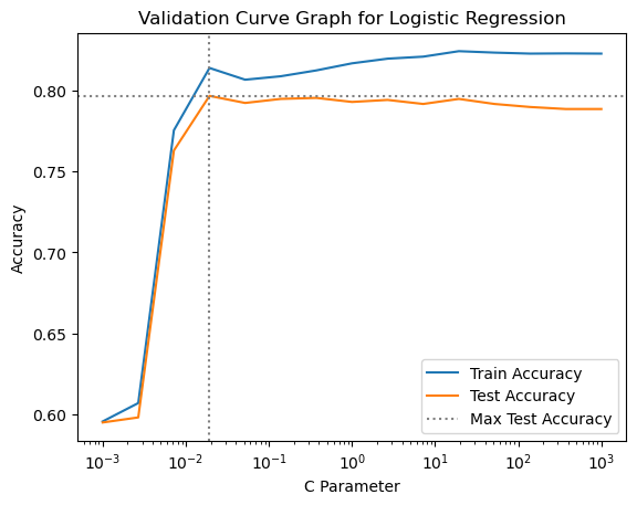
The initial parameter range we chose for the logistic regression grid searches is fine, as the best parameter setting is near the middle of the range. It looks like the peak performance is between \(10^{-3}\) and \(10^2\), so we will focus the search on that range of C values by re-defining the parameter grid and grid search before running the nested cross validation.
# Re-define the parameter grid
pgrid_lreg = {'cls__C': np.logspace(-3, 2, 20)}
# Re-define the grid search
gs_lreg = GridSearchCV(estimator = pipe_lreg,
param_grid = pgrid_lreg,
cv = rskf_3x6f,
n_jobs = -1,
scoring = 'accuracy')Now we can run the nested cross validation. A nested cross validation is implemented with a cross_validate() function in which the estimator is a grid search. A timer has been added to the code, using the perf_counter() function from the time module.
# Start the timer
start = time.perf_counter()

# Perform the nested cross validation for logistic regression
lreg_gen_scores = cross_validate(estimator = gs_lreg,
                                 X = features,
                                 y = target,
                                 cv = rskf_3x6f,
                                 scoring = 'accuracy')
# Stop the timer
end = time.perf_counter()

# Print out message with the elapsed time
print(f"Elapsed time is {end - start:0.2f} seconds")
Elapsed time is 86.91 secondsNext, we calculate the mean and standard deviation of test-fold performance for logistic regression. These represent our estimate of generalization performance for the logistic regression algorithm on this data. After we go through a similar process for K-nn we can compare the estimated generalization performance of logistic regression and K-nn on the Titanic data.
print(f"lreg mean test score: {np.mean(lreg_gen_scores['test_score'])}")
print(f"lreg std test score: {np.std(lreg_gen_scores['test_score'])}")
lreg mean test score: 0.8000640934339839
lreg std test score: 0.0342970857538839710.6.4 K-Nearest Neighbors
Now we will conduct a nested cross validation to estimate generalization performance for the K-Nearest Neighbors model on the Titanic data.
The code cell below sets up the column transformer, pipeline, parameter grid, cross validation splitter, and grid search.
# Make column transformer to do preprocessing
ct_knn = ColumnTransformer([
    ('mm_scale', MinMaxScaler(), num_features),
    ('one_hot', OneHotEncoder(handle_unknown = 'ignore'), cat_features)
])

# Make pipeline to combine preprocessing with estimator
pipe_knn = Pipeline([
    ('pre', ct_knn),
    ('cls', KNeighborsClassifier())
])

# Define parameter grid
pgrid_knn = {'cls__n_neighbors': range(1, 100, 4)}

# Set up a splitter for 3 x stratified 6-fold cv
rskf_3x6f = RepeatedStratifiedKFold(n_splits = 6, n_repeats = 3)

# Define grid search
gs_knn = GridSearchCV(estimator = pipe_knn,
                      param_grid = pgrid_knn,
                      cv = rskf_3x6f,
                      n_jobs = -1,
                      scoring = 'accuracy',
                      return_train_score = True)
10.6.5 Run the grid search once to check if the parameter range is appropriate
Below we run the grid search once to check to see if the best parameter setting is within the range we chose when we set up the grid search.
gs_knn.fit(X_train, y_train)GridSearchCV(cv=RepeatedStratifiedKFold(n_repeats=3, n_splits=6, random_state=None),
estimator=Pipeline(steps=[('pre',
ColumnTransformer(transformers=[('mm_scale',
MinMaxScaler(),
['Age',
'SibSp',
'Parch']),
('one_hot',
OneHotEncoder(handle_unknown='ignore'),
['Sex',
'Pclass',
'Embarked'])])),
('cls', KNeighborsClassifier())]),
n_jobs=-1, param_grid={'cls__n_neighbors': range(1, 100, 4)},
return_train_score=True, scoring='accuracy')In a Jupyter environment, please rerun this cell to show the HTML representation or trust the notebook. On GitHub, the HTML representation is unable to render, please try loading this page with nbviewer.org.
Parameters
| estimator | Pipeline(step...lassifier())]) | |
| param_grid | {'cls__n_neighbors': range(1, 100, 4)} | |
| scoring | 'accuracy' | |
| n_jobs | -1 | |
| refit | True | |
| cv | RepeatedStrat...om_state=None) | |
| verbose | 0 | |
| pre_dispatch | '2*n_jobs' | |
| error_score | nan | |
| return_train_score | True |
Parameters
| transformers | [('mm_scale', ...), ('one_hot', ...)] | |
| remainder | 'drop' | |
| sparse_threshold | 0.3 | |
| n_jobs | None | |
| transformer_weights | None | |
| verbose | False | |
| verbose_feature_names_out | True | |
| force_int_remainder_cols | 'deprecated' |
['Age', 'SibSp', 'Parch']
Parameters
| feature_range | (0, ...) | |
| copy | True | |
| clip | False |
['Sex', 'Pclass', 'Embarked']
Parameters
| categories | 'auto' | |
| drop | None | |
| sparse_output | True | |
| dtype | <class 'numpy.float64'> | |
| handle_unknown | 'ignore' | |
| min_frequency | None | |
| max_categories | None | |
| feature_name_combiner | 'concat' |
Parameters
| n_neighbors | 49 | |
| weights | 'uniform' | |
| algorithm | 'auto' | |
| leaf_size | 30 | |
| p | 2 | |
| metric | 'minkowski' | |
| metric_params | None | |
| n_jobs | None |
gs_knn.best_params_{'cls__n_neighbors': 49}# Extract the grid search results to a DataFrame
results_knn = pd.DataFrame(gs_knn.cv_results_)
# Create the validation curve plot with matplotlib
plt.plot(results_knn['param_cls__n_neighbors'],
results_knn['mean_train_score'])
plt.plot(results_knn['param_cls__n_neighbors'],
results_knn['mean_test_score'])
plt.axhline(y = max(results_knn['mean_test_score']),
color = 'gray',
linestyle = ':')
plt.axvline(x = results_knn['param_cls__n_neighbors'][results_knn['mean_test_score'].idxmax()],
color = 'gray',
linestyle = ':')
# Flip the x-axis limits so that flexibility increases from left to right
plt.xlim(max(results_knn['param_cls__n_neighbors']),
min(results_knn['param_cls__n_neighbors']))
plt.title("Validation Curve Graph for K-nn")
plt.xlabel("Number of Neighbors")
plt.ylabel("Accuracy")
plt.legend(["Train Accuracy", "Test Accuracy", "Max Test Accuracy"],
loc="best");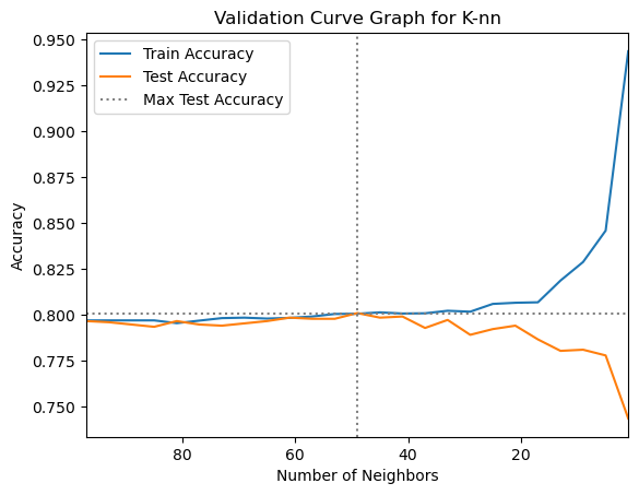
The initial parameter ranges we chose for the grid search looks a little wide. It looks like the peak performance is when number of neighbors is between 35 and 70, so we will focus the search on that range of n_neighbors values by re-defining the parameter grid and grid search before running the nested cross validation.
# Re-define parameter grid
pgrid_knn = {'cls__n_neighbors': range(35, 71)}

# Re-define grid search
gs_knn = GridSearchCV(estimator = pipe_knn,
                      param_grid = pgrid_knn,
                      cv = rskf_3x6f,
                      n_jobs = -1,
                      scoring = 'accuracy')
Now we can run the nested cross validation. A nested cross validation is implemented with a cross_validate() function in which the estimator is a grid search. A timer has been added to the code, using the perf_counter() function from the time module.
# Start the timer
start = time.perf_counter()

# Perform the nested cross validation for K-nn
knn_gen_scores = cross_validate(estimator = gs_knn,
                                X = features,
                                y = target,
                                cv = rskf_3x6f,
                                scoring = 'accuracy')

# Stop the timer
end = time.perf_counter()

# Print message with the elapsed time
print(f"Elapsed time is {end - start:0.2f} seconds")
Elapsed time is 105.01 secondsNext, we calculate the mean and standard deviation of test-fold performance for K-nn. These represent our estimate of generalization performance for the K-nn algorithm on this data. We can compare them to the estimated generalization performance of logistic regression on the Titanic data.
print(f"knn mean test score: {np.mean(knn_gen_scores['test_score'])}")
print(f"knn std test score: {np.std(knn_gen_scores['test_score'])}")
knn mean test score: 0.7936310117267246
knn std test score: 0.04020077703254578610.6.6 Perform grid search on model with best estimated generalization performance to set parameters
These models have very similar estimated generalization performance, but the logistic regression is slightly better. Let’s go ahead and move forward with the logistic regression model. Because the performance of the two models is so similar you may see a different result if you re-run this code.
The final step in our model building process is to run a new grid search for the best model using all our labeled data. When it finishes the grid search will retrain the model with the best parameters on all the labeled data, and it will then function as an estimator that we can use to make predictions for other Titanic passengers.
gs_lreg.fit(features, target)GridSearchCV(cv=RepeatedStratifiedKFold(n_repeats=3, n_splits=6, random_state=None),
estimator=Pipeline(steps=[('pre',
ColumnTransformer(transformers=[('poly_std',
Pipeline(steps=[('poly',
PolynomialFeatures(degree=3,
include_bias=False)),
('std',
StandardScaler())]),
['Age',
'SibSp',
'Parch']),
('one_hot',
OneHotEncoder(),
['Sex',
'Pclass',
'Embarked'])])),
('cls',
LogisticRegression(max_iter=2000))]),
n_jobs=-1,
param_grid={'cls__C': array([ 0.1 , 0.14384499, 0.20691381, 0.29763514,
0.42813324, 0.61584821, 0.88586679, 1.27427499,
1.83298071, 2.6366509 , 3.79269019, 5.45559478,
7.8475997 , 11.28837892, 16.23776739, 23.35721469,
33.59818286, 48.32930239, 69.51927962, 100. ])},
scoring='accuracy')In a Jupyter environment, please rerun this cell to show the HTML representation or trust the notebook. On GitHub, the HTML representation is unable to render, please try loading this page with nbviewer.org.
Parameters
| estimator | Pipeline(step..._iter=2000))]) | |
| param_grid | {'cls__C': array([ 0.1 ...100. ])} | |
| scoring | 'accuracy' | |
| n_jobs | -1 | |
| refit | True | |
| cv | RepeatedStrat...om_state=None) | |
| verbose | 0 | |
| pre_dispatch | '2*n_jobs' | |
| error_score | nan | |
| return_train_score | False |
Parameters
| transformers | [('poly_std', ...), ('one_hot', ...)] | |
| remainder | 'drop' | |
| sparse_threshold | 0.3 | |
| n_jobs | None | |
| transformer_weights | None | |
| verbose | False | |
| verbose_feature_names_out | True | |
| force_int_remainder_cols | 'deprecated' |
['Age', 'SibSp', 'Parch']
Parameters
| degree | 3 | |
| interaction_only | False | |
| include_bias | False | |
| order | 'C' |
Parameters
| copy | True | |
| with_mean | True | |
| with_std | True |
['Sex', 'Pclass', 'Embarked']
Parameters
| categories | 'auto' | |
| drop | None | |
| sparse_output | True | |
| dtype | <class 'numpy.float64'> | |
| handle_unknown | 'error' | |
| min_frequency | None | |
| max_categories | None | |
| feature_name_combiner | 'concat' |
Parameters
| penalty | 'l2' | |
| dual | False | |
| tol | 0.0001 | |
| C | np.float64(2.636650898730358) | |
| fit_intercept | True | |
| intercept_scaling | 1 | |
| class_weight | None | |
| random_state | None | |
| solver | 'lbfgs' | |
| max_iter | 2000 | |
| multi_class | 'deprecated' | |
| verbose | 0 | |
| warm_start | False | |
| n_jobs | None | |
| l1_ratio | None |
gs_lreg.best_params_{'cls__C': np.float64(2.636650898730358)}Now we can use gs_lreg as our final model to make predictions on new data